Guro Dørum and Mariam Mjærum Bouzga

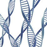
Urn models have a long tradition in probability and statistics. Jacob Bernoulli studied urn models as early as the 17th century to determine the proportions of differently colored balls based on a sample drawn from the urn. The basic idea is that we have an urn containing balls in two or more different colors, balls are drawn from the urn, and their colors are recorded. If a ball is returned to the urn after its color has been recorded, we call it drawing with replacement. If the ball is not returned to the urn we call it drawing without replacement. Figure 1 illustrates a simple urn model. In this paper we will use urns to describe concepts in forensic genetics, starting with an explanation of some basic concepts within this field.

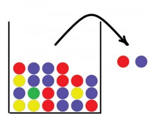
Figure 1. Sampling from an urn

Basic Forensic Genetics

Forensic genetics involves the use of DNA to solve criminal cases, paternity cases, identification cases with missing persons, and disaster victim identification. In this paper, we will focus only on criminal cases. DNA was first used as evidence in a criminal case in 1987 and has since grown to become one of the most important forensic investigation tools. In the legal system, DNA is often regarded as the most reliable type of evidence.

All humans, except identical twins, are expected to differ in their genetic code. (Actually, even identical twins may differ a little in their DNA). However, more than 99% of the genetic code is identical in all humans. Parts of the DNA with high variability between individuals have been chosen as genetic markers for use in forensic genetics. More than 98% of the human DNA is non-coding, meaning that it does not encode protein sequences. Non-coding DNA is believed to have been less exposed to evolutionary selection than DNA that encodes proteins. The most common type of genetic markers used in forensics, STR markers, are chosen from among non-coding DNA sequences. By studying a quite small number of genetic markers, we are able to distinguish between individuals with great reliability. The standard within forensic investigation in Europe today is to evaluate 16 STR markers, plus one marker to determine sex.

In all cells except sex cells, humans have two copies of their DNA. One copy is on chromosomes inherited from the mother and one is on chromosomes inherited from the father. We call each copy of a DNA sequence an allele. The STR markers are DNA sequences with a high number of different alleles in the population. An individual may have two identical alleles in a marker (the individual is homozygous) or two different alleles (the individual is heterozygous). The two alleles in a genetic marker together make up the individual’s genotype. The combination of genotypes for all genetic markers makes up the individual’s genetic profile. For example, 1/1 denotes the genotype for one marker with two copies of the allele 1. Further, 1/1, 2/3 denote a genetic profile for two markers, where the second marker has the alleles 2 and 3. Note that this individual is homozygous in the first marker and heterozygous in the second marker.

The lack of evolutionary selection on STR markers implies that they tend to have a high variability in the population, making it easier to differentiate between individuals. The allele frequencies play an important role in the calculation of the strength of the DNA evidence, as will be explained later.

The STR markers are usually situated on different chromosomes; if they are on the same chromosome, they are so far apart that they will not be inherited together during the meiosis (the process of making sex cells). In a statistical context, it means that the individual markers can be regarded as independent of each other: a person’s genotype at one marker gives no information about the person’s genotype at another marker. Compared to other types of evidence used in forensics, such as fingerprints and characteristics of teeth (forensic odontology), DNA is unique in the sense that there is so much independent information available.

DNA Databases

To understand how rare a genetic profile is, it is necessary to understand the frequency of different alleles that are in the population of interest. These allele frequencies are calculated from a DNA database that contains a sample of genetic profiles from a population. Population here may refer to a whole nation or a particular ethnic group. The differences in allele frequencies may be quite large between major populations, while there are small differences between subpopulations.

Hardy-Weinberg

The Hardy-Weinberg law states that allele frequencies in a genetic marker are independent from one another. In other words, the allele inherited from your mother is independent of the allele inherited from your father. It is assumed that your parents have not chosen each other based on their genotypes and that there is random mating in the population. Hardy-Weinberg implies that we can follow the rules of independent probabilities when calculating probabilities for genotypes. If a marker has two alleles, 1 and 2, with frequencies p₁ and p₂, we can calculate the genotype probabilities as

.

The assumption of random mating may not be entirely true, and in practice the genotype probabilities are usually corrected to account for subpopulation effects. For simplicity, however, we will assume Hardy-Weinberg in all calculations in this paper.

Likelihood Ratio

The most common statistical analysis of DNA evidence involves calculating a likelihood ratio (LR). The likelihood ratio evaluates the probability of the evidence (E) on the basis of two alternative hypotheses—a prosecution hypothesis (H_p) and a defense hypothesis (H_d). The likelihood ratio is

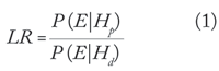
where P (E|H_p) is the conditional probability of the evidence given the prosecution hypothesis, and P (E|H_d) is the conditional probability of the evidence given the defense hypothesis. If the likelihood ratio is larger than 1, the evidence supports the prosecution hypothesis, while if it is smaller than 1 the evidence supports the defense hypothesis. A likelihood ratio of 1 means that the evidence gives equal support to both hypotheses.

Case Example

A woman has been raped and a suspect has provided a reference DNA sample. Based on a vaginal swab from the victim, sperm cells have been separated from the victim’s epithelial cells, and DNA has been extracted from the sperm cells as evidence. The goal is to determine whether the suspect is the contributor to the DNA in the evidence sample. Reference samples also are taken from the victim herself and the victim’s partner, in order to exclude these as contributors to the evidence. (DNA from the victim would be observed only if the sperm cells have not been completely separated from the epithelial cells.)

Table 1 shows the alleles found in the evidence and in the reference samples of the suspect, the victim’s partner, and the victim. The first row in the table (AM) is the sex marker that identifies the individuals as male (X/Y) or female (X/X). A quick inspection of the table shows that the suspect fits with the evidence alleles at all markers except D3S1358. In this marker the evidence only shows the allele 15, while the suspect also has the allele 16. The alleles of the victim’s partner fit with the evidence alleles in the marker D3S1358, but do not fit in many of the other markers. Since there is not a complete match between the suspect and the evidence, we cannot exclude the possibility that there is a third person, other than the suspect and the victim’s partner, who is the contributor to the evidence. There is, however, a possibility that the suspect’s allele that is missing in the evidence could have “dropped out.” This phenomenon, and how to handle it, is described in a separate subsection later in this article. For now, we choose to leave D3S1358 out of the statistical calculations.

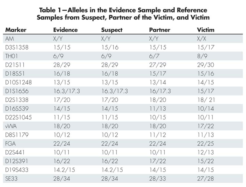
Table 1-Alleles in the Evidence Sample and Reference Samples from Suspect, Partner of the Victim, and Victim

The prosecution proposes the hypothesis H_p: The DNA in the evidence comes from the suspect. The defense could propose that the DNA comes from the partner of the victim since they are known to have had sexual intercourse. But considering that the partner does not fit the evidence very well, the defense is better off suggesting the hypothesis H_d: The DNA in the evidence comes from an unknown person.

Table 2 gives allele frequencies for the two markers D3S1358 and TH01. Box 1 shows how to compute the likelihood ratio for the marker TH01. The likelihood ratios for the individual markers (excluding D3S1358) can be multiplied to produce the total likelihood ratio of 7.46 x 10²⁷. The large likelihood ratio implies that the evidence gives very strong support to the prosecution hypothesis that the DNA originated from the suspect.

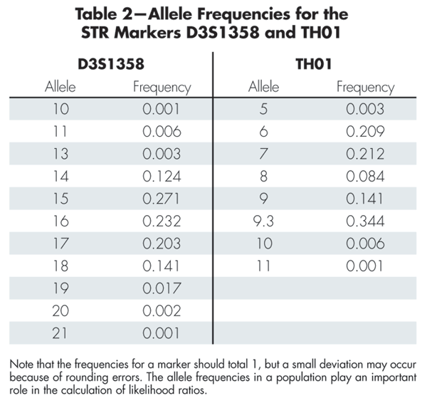
Table 2-Allele Frequencies for the STR Markers D3S1358 and TH01

Urn Models in Forensics

Allele frequencies

Allele frequencies are essential to estimate the strength of the DNA evidence in crime cases. These frequencies are taken from a DNA database that represents the population of interest, usually the population that the suspect comes from. The number of individuals in the database is usually very small compared to the number of individuals in the population. We can imagine an urn that contains all alleles in the population, where the different alleles are represented by different colored balls. A DNA database is a small sample of balls from this urn that’s used to determine the proportion of different colors in the urn.

Sometimes forensic scientists discover alleles not represented in the DNA database. In other words, the sample from the population urn was too small to discover all colors in the urn. As a consequence, these alleles have no frequency estimates, yet we cannot treat the alleles as having a probability 0 of occurring.

So how can we avoid this problem? A solution that is sometimes used is a Bayesian approach that assigns prior probabilities to the allele frequencies. We will describe the approach here with the use of urns. Figure 2 shows three urns. The first urn represents the prior distribution. The balls in this urn may represent the alleles in a DNA database for a population similar to the one we are interested in. This “prior urn” contains balls with all the colors needed to overcome the problem of encountering alleles with probability 0 of occurring; each possible allele must be represented at least once. The number of balls in the prior urn reflects how much weight we want to put on the prior distribution. By increasing the number of balls in the urn we increase the weight on the prior information.

Figure 2. Estimating allele frequencies with the Bayesian approach. All the balls in the prior urn and a sample of balls from the population urn (the observed data) are mixed together in the posterior urn. By counting the number of balls of each color in the posterior urn we get the allele frequency estimates. Note that if we had not used the balls in the prior urn we would not have a frequency estimate for the green ball, since no green balls were included in the sample from the population urn.

The second urn, the “population urn,” contains all alleles in the population of interest (there are too many for us to count all). We draw a number of balls from the population urn and take all balls from the prior urn and mix them together in a third urn that we call the “posterior urn.” The posterior urn is the DNA database for the population of interest. By counting the number of balls of each color in the posterior urn, we can estimate the population allele frequencies.

Drop-in and drop-out

Drop-in and drop-out are phenomena typically associated with low-level or degraded DNA samples. Drop-in alleles are contaminant alleles that have dropped into the sample. A drop-in allele is revealed when it fails to reproduce if the same sample is analyzed several times. Drop-in may explain one or more alleles in the evidence that are not in the reference profiles; however it is a rare event. Drop-out alleles are alleles that have dropped out of the sample. Drop-out occurs when an allele cannot be visualized in the profile; for example, because it fails to amplify during PCR (polymerase chain reaction). It may have completely dropped out or its signal may be too weak to be distinguished from noise. It is most often observed when one of the alleles of a heterozygous marker cannot be visualized, and the result may be that it is misinterpreted as a homozygous marker. One or more alleles may have dropped out of the sample, and drop-out may therefore explain alleles in the reference profiles not found in the evidence.

Simulation of genotypes with drop-in and drop-out is illustrated in Figure 3. Two balls drawn from a population urn represent the genotype. In Figure 3(a) a drop-out happens when one of the balls falls out of the sample before its color is recorded. Figure 3(b) illustrates a drop-in when a ball drawn from a different urn falls into the sample. It is possible that both alleles in a genotype drop out and that more than one allele drops in.

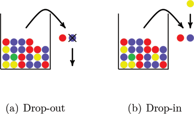
Figure 3. A drop-out allele modeled as a ball that falls out of the sample before its color is recorded and a drop-in allele modeled as a ball drawn from another urn that falls into the sample.

If we take the probability of drop-in and drop-out into account, it may have considerable impact on the likelihood ratio. Recall that in the case example we chose to leave the marker D3S1358 out of the statistical calculations because the suspect did not fit with the evidence in this marker. Box 2 explains how we can still compute the likelihood ratio for the marker D3S1358 if we factor in the probability of drop-in and drop-out. Including drop-in and drop-out probabilities different from 0 also affects the remaining markers. Under the defense hypothesis there are more possibilities for the unknown individual. If we recalculate the likelihood ratio for all markers with drop-out probability 0.1 and drop-in probability 0.05, the overall likelihood ratio is 4.78 x 10²⁷. The likelihood ratio is slightly smaller compared to when D3S1358 was left out of the calculation. This is both due to the introduction of more uncertainty when we allow for drop-in and drop-out, and because the overall likelihood ratio is multiplied by the factor 0.8307 when the marker D3S1358 is included. The likelihood ratio still gives strong support to the prosecution hypothesis.

Likelihood ratio with drop-in and drop-out by simulation

The formula for calculating likelihood ratios quickly gets complex when probabilities of drop-in and drop-out are introduced. Box 2 shows a very simple example, and often we will encounter much more complicated calculations. We will therefore illustrate how urn models can be used to estimate likelihood ratios with drop-in and drop-out without considering any complicated formula. By doing a large number of draws from the urn, we simulate evidence samples that could have been observed. Finally, we count how many times the alleles in the simulated evidence correspond to the observed evidence. We will only consider the genetic marker D3S1358, but the approach can easily be extended to several markers. The simulation procedures for estimating the probability of the evidence given the prosecution hypothesis, P (E | H_p), and the probability of the evidence given the defense hypothesis, P (E | H_d ), are similar. The only difference is the genotype we begin with. For P (E | H_p), our starting point in each simulation is the suspect’s genotype 15/16, while for P (E | H_d ), we draw for each simulation a genotype from an urn representing the population alleles. The procedure is as follows:

1. Find the starting genotype, either the suspect’s genotype (H_p) or a random genotype from the population urn (H_d).

2. With a given probability, one or both alleles drop out of the genotype, and one or more alleles drop into
the genotype.

3. Repeat steps 1 and 2 10,000 times.

4. Count how many times we end up with a sample that contains only the allele 15 and divide this number by 10,000.

Step 4 gives us the probability of the evidence given the hypothesis. The estimated probability of the evidence given the prosecution hypothesis is P (E | H_p) = 0.0866, and the estimated probability of the evidence given the defense hypothesis is P (E | H_d ) = 0.1035. The likelihood ratio is 0.0866/0.1035=0.8367, approximately the same number as we got with the likelihood ratio formula in Box 2.

Further Reading

Buckleton, J., C. M. Triggs, and S. J. Walsh (editors). 2005. Forensic DNA evidence interpretation. CRC Press.

Weir, B. 1995. DNA statistics in the Simpson matter. Nature Genetics 11:365–368.

About the Authors

Mariam Mjærum Bouzga is a forensic expert in the department of forensic genetics at the Norwegian Institute of Public Health. She earned her BS and MA in biochemistry at the University of Oslo. She is working on her PhD in forensic genetics and epigenetics.

Guro Dørum is a postdoc in the biostatistics group in the department of chemistry, biotechnology, and food science at the Norwegian University of Life Sciences, where she also earned her BS and MA in bioinformatics and PhD in applied statistics. Her research interests involve developing statistical methods for forensic genetics and genomics.

Back To Top