
Measuring Player Contributions in Hockey

Hockey is a popular sport due to the continuous nature of play and frequent changes of players on the ice that leads to a fast pace of gameplay. Adding to the excitement is the relatively high frequency of scoring opportunities, but the relatively low frequency of scoring events. However, these same intrinsic properties of the sport make it difficult to quantify the performance of individual players. Specifically, there is a lot of interest in measuring the contribution of each player to goal scoring, which is not easy given the continuity of play, frequent line changes, and the infrequency of goals.
The historical standard by which the overall contribution of a hockey player is measured is plus-minus (or +/–): each player on the ice gets a +1 when a goal is scored by their team and a –1 when a goal is scored against their team. These positives and negatives are aggregated over an entire season for each player, so that the plus-minus for a player is the total number of goals scored by their team minus the total number of goals scored by their opponents while that player was on the ice.
Plus-minus is intuitive and easy to calculate from game data, but has some obvious disadvantages. First and foremost, plus-minus for any particular player does not just depend on their contribution but also the contributions of their teammates and their opponents. Since the set of teammates and opponents that each player is matched with on-ice is different, the plus-minus measure for individual players is inherently polluted. Plus-minus is also not standardized for comparing players that spend very different amounts of time on the ice.
We can view plus-minus for a player from a statistical perspective as a marginal player effect that averages over the context experienced by that particular player. What we would rather have is a partial player effect: What does that particular player contribute to goal scoring/prevention on top of the contributions of their teammates and opponents? Hence, a regression model for estimating partial effects is a natural approach to improving upon plus-minus.
Within the past 10 years, linear regression approaches have been used to estimate partial effects of individual players in basketball and hockey. Basketball is similar to hockey in the sense that both sports consist of continuous fast-paced play with frequent player substitutions. However, basketball is very different from hockey in the sense that (1) scoring events are much less frequent in hockey and (2) players tend to substitute together as “lines” in hockey. Both of these aspects complicate the estimation of individual player effects in hockey.
To address issue #1, the infrequency of scoring events, it is more appropriate to model player effects on the log-odds of a goal being scored rather than a linear regression on total goals scored. Specifically, we can model the probability pi that a given goal i was scored by the home team,
![]()
where β = [β1 · · · βnp]’ is the vector of partial plus-minus effects for each of np players in hockey, with {hi1 . . . hi6}, {ai1 . . . ai6} being the indices on β corresponding to home-team (h) and away-team (a) players on the ice for goal.
Issue #2, that players tend to substitute together as “lines” in hockey, is problematic for regression modeling since it makes it harder to separate the contributions of individual players if they are always on the ice with the same set of teammates. In statistical terms, the indicator variables for players on the same line will be highly collinear, which could lead to unstable estimates of their partial plus-minus effects in the above equation.
Regularization is a popular way for promoting stability in high-dimensional regression models with collinearity. From the classical perspective, we can include a penalty term into the regression optimization that shrinks the optimal estimates of β toward zero. Common regularization strategies are ridge regression, which places an L2 penalty, and lasso regression, which places an L1 penalty, on the partial effects β. From the Bayesian perspective, these penalty terms correspond to particular prior distributions on the parameters β. The L2 penalty corresponds to a Gaussian prior distribution centered at zero for β, whereas the L1 penalty corresponds to a Laplace prior distribution centered at zero for β.
When the number of predictor variables is large, the L1 penalty (lasso regression) is especially popular, since it leads to optimal estimates βˆ where many of the βˆ i are set to exactly zero. This characteristic eases interpretation of the regression model since we can focus attention on the small subset of selected variables with non-zero estimates βˆ i. In the context of player performance in hockey, the L1 penalty allows a small number of highly effective players to stand out from their teammates and opponents.
I have been involved in two recent papers that take a regularized approach to estimate player performance in hockey, and I will outline some features of both approaches. The data for these papers, from www.nhl.com, consists of all games over five seasons (2007–2011), which contains approximately 18,000 even-strength goals and around 1,500 players. In both approaches, we restrict ourselves to even-strength goals to remove the difficulty of handling power-play situations in which one team is playing with fewer players than the other.
The first paper is Bobby Gramacy, Shane Jensen, and Matt Taddy’s 2013 Journal of the Quantitative Analysis of Sports paper, “Estimating Player Contribution in Hockey with Regularized Logistic Regression.” Here, we implement the logistic regression model outlined above, but we also consider overall team effects on goal scoring. We use an L2 penalty term on the partial team effects, which encourages every team to have a small, but non-zero, effect on goal scoring. We use an L1 penalty on the partial effects of each player, so the model will pick out a subset of players who stand out relative to their team and the other players in the data set.
In Figure 1, we give all players who were estimated by our model to have a substantial effect on scoring. In other words, we examine only the players with non-zero partial player effects. This plot actually compares estimated player effects from two models: the model with both player and team effects and the model with just player effects.

Figure 1. Comparing player effects from two models: the model with both player and team effects and the model with just player effects. The black dots are player effects for the model with both player and team effects. A line comes out of each dot that links to the player effect for the model without the team effects. Red lines indicate decreased effects in the model that includes team, whereas blue lines indicate increased effects in the model that includes team. Players with coefficients estimated as zero under both models are not shown.
The black dots in the plot are the estimated player effects for the model with both player and team effects. A line comes out of each dot that links to the estimated player effect for the model without the team effects. Red lines are given to players who have decreased effects in the model that includes team, whereas blue lines are given to players who have increased effects in the model that includes team.
Overall, we see that using an L1 penalty has led to the selection of a small number, about 100 out of the original 1,500, of players who have a non-zero player effect in either model. We highlight several notable players with red text. The best player according to our model is Pavel Datysuk, who stands far above the other players in model with team effects, and his player effect doesn’t change in the model without team effect. Craig Adams and Radek Bonk stand out as the worst players according to our model with team and player effects. However, their player effects do improve when the team effects are not included.
In fact, we see many players who have substantially different player effects depending on whether team effects are included in the model. Sidney Crosby has a player effect that drops after accounting for his team, though he still has a positive contribution in both models. Zdeno Chara has a positive player effect in the model without team effects, but his player effect drops to zero after having accounted for his strong Boston Bruins team. Dwayne Roloson has a zero effect in the model without team effects, but a strong positive effect when having accounted for the weak teams he played on (Tampa Bay Lightning, New York Islanders, Edmonton Oilers, and Minnesota Wild).
In Figure 2, we compare our partial player effects to the traditional plus-minus statistic for all players who had a non-zero player effect in our model with team effects included. The points are colored and labeled according to the position of that player (C = center, L = left wing, R = right wing, D = defense, G = goalie). We also give the estimated team effects for some teams compared to their aggregate team plus-minus.
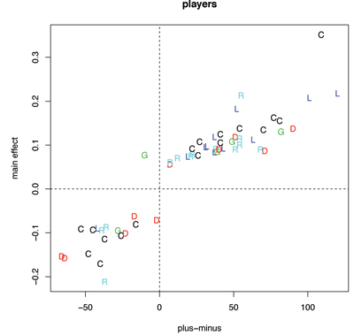
Figure 2. Left: Comparing player effects to the traditional plus-minus statistic for all players who had a non-zero player effect. Plot symbols give positional information: C = center, L = left wing, R = right wing, D = defense, and G = goalie. Right: Comparing team effects to their aggregate plus-minus values.
The positive association between traditional plus-minus and our partial player effects indicates general agreement between the two measures, but there are some interesting discrepancies as well. For example, we disagree with plus-minus in terms of the best player in hockey. Datysuk stands well above all others according to our approach, but Alexander Ovechkin has the largest plus-minus. Roloson has a negative plus-minus value, but is estimated by our model to have a large positive partial effect. Roloson’s negative plus-minus could be driven by his weak teams (TB, NYI, EDM, and MIN), which all have negative team plus-minus and negative team effects according to our model.
The second paper I will describe is “Competing Process Hazard Function Models for Player Ratings in Ice Hockey” by Andrew Thomas, Samuel Ventura, Shane Jensen, and Stephen Ma, which will appear in the Annals of Applied Statistics. This paper uses an additional season of data (2012) and takes a different approach to goal scoring. Goals by the home team versus goals by the away team are set up as two competing processes. Each of these processes is specified as a Cox proportional hazards model where the scoring rates in each process are functions of the particular players on the ice.
One benefit of this two-process approach is we can separate the offensive vs. defensive contributions of each player. Each process also can account for all the time on the ice in which goals are not scored, whereas the first approach ignores this non-goal portion of the game. The same issue of collinearity between players is present in this second model, and so regularization is again needed to help stabilize our estimated partial offensive and defensive effects for each player. In this paper, we use a combination of the L1 and L2 penalties commonly called “the elastic net.”
The offensive and defensive effects for each player can be combined into a “net goals contributed” over an average player. In figure 3, we compare the net goals contributed for each player from our model to the traditional plus-minus measure.
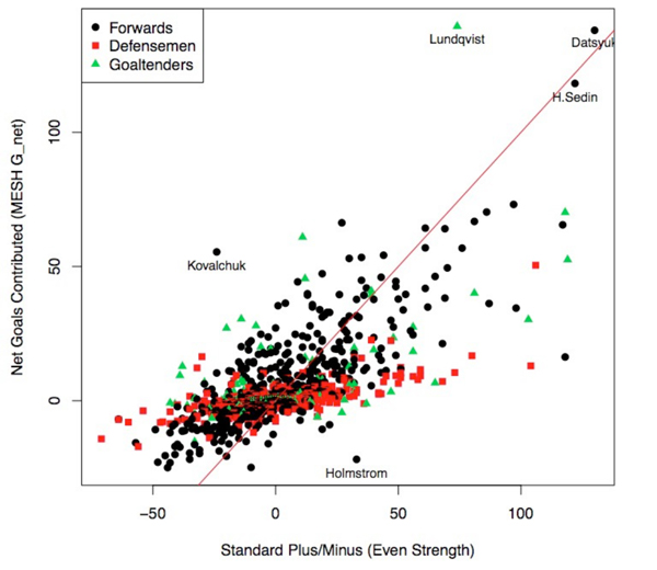
Figure 3. Comparing net goals contributed from our model to the traditional plus-minus measure for each player. Different symbols are used for forwards versus defensemen versus goaltenders. Several outlying players are labeled.
We see that Datysuk stands out as one of the best players in hockey, which agrees with the results of the first paper. However, Datysuk does not stand out alone in this analysis; he is joined by Henrik Sedin and goaltender Henrik Lundqvist. Lundqvist is given a substantial boost in our model compared to traditional plus-minus. Ilya Kovalchuk is also a substantial increase in our model relative to his plus-minus, whereas Tomas Holmstrom sees a substantial decrease in our model relative to his plus-minus.
Both papers are rather complicated statistical approaches to the analysis of player performance in hockey. This sophistication was required by two unique challenges in the quantitative study of hockey: the relative infrequency of scoring events and the collinearity between teammates who play together on the same line. In both cases, our approaches were able to detect subtle and interesting effects that would be masked by the standard plus-minus metric.
Much work remains to be done in the quantitative study of hockey. Power-play goals need to be added into our analysis in a principled way. Incorporating more detailed information about shots and passes as well as other on-ice events could also give a more resolute picture of each player’s contribution. There have already been some statistics introduced for shots, with Corsi and Fenwick being the most notable. Finally, there needs to be more dialogue with the decisionmakers in professional hockey that stand to benefit from these quantitative analyses of player performance.
Further Reading
Gramacy, R.B., S.T. Jensen, and M. Taddy. 2013. “Estimating player contribution in hockey with regularized logistic regression.” Journal of Quantitative Analysis in Sports 9:97–111.
Thomas, A.C., S.L. Ventura, S.T. Jensen, and S. Ma. 2013. Competing process hazard function models for player ratings in ice hockey. Accepted for publication in the Annals of Applied Statistics.
About the Author
Shane Jensen is an associate professor of statistics in the Wharton School at the University of Pennsylvania, where he has been teaching since completing his PhD at Harvard University in 2004. Jensen has published more than 40 academic papers in statistical methodology for a variety of applied areas, including molecular biology, psychology, and sports. He maintains an active research program in developing sophisticated statistical models for the evaluation of player performance in baseball and hockey.


