
Easy to Criticize, Harder to Verify: Fourth and Goal in Post-2011 NFL Overtime

Quarterback Matt Flynn had been Aaron Rodgers’ backup for four seasons in Green Bay before signing on with Seattle in 2012 with the hope of being their starting quarterback. When Rodgers went down with a broken collarbone in week nine of the 2013 season, the Green Bay Packers (GB) brought Flynn back to help out. On week 13, in a home game against the Minnesota Vikings (MN), GB turned to Flynn to keep their playoff hopes alive. Down by 16 in the fourth quarter, Flynn led a heroic comeback to tie the game and send it to overtime.
Until 2012, overtime had a sudden-death format, which meant the game was won by the first team to score. This gave a huge advantage to the team that won the coin toss. Previous research by Chris Jones found that 64% of overtime games from 2004-2008 were won by the team that received the overtime kickoff. To mitigate this dependence on a coin flip, the NFL modified the overtime format so that the first team to possess the ball cannot just kick a field goal on the opening drive and win the game. The team must either score a touchdown, or kick a field goal and then stop the other team from scoring on its subsequent possession. Should the teams trade field goals, or if the first-possession team fails to score on the opening drive, the game reverts to the sudden-death format.
This slight change to the format strongly influences decisionmaking of the first-possession team. Should the team aggressively pursue the winning touchdown, or settle for the more easily acquired field goal and bet on their defense to make one last stop?
With these new rules governing the game, GB received the opening overtime kickoff and drove down to the MN two-yard line. Facing fourth down and goal, Head Coach Mike McCarthy had to decide what to do with the last play of the drive: kick the field goal and bank on a defensive stop, or go for the touchdown and win. GB had a strong running game that year with the addition of rookie running back Eddie Lacy, and had already converted two fourth downs in the game. GB also had the fan-favorite concept of momentum on their side, and should GB fail to score, MN would be pinned back near their own goal line, making a scoring drive very difficult.
Yet to the chagrin of many Packers fans, McCarthy sent out the field-goal unit, putting his team up three and giving Minnesota at least one more chance to win the game. The GB defense could not hold, and MN answered with a field goal, leaving just less than four minutes to play. Neither team scored in those last minutes, so the game ended in a tie—a relatively rare occurrence for an NFL game.
Such a visible decision as McCarthy’s fourth-and-goal choice to kick the field goal warranted, and received, a lot of discussion in the sports-talk world. The popular opinion was that GB should have gone for the touchdown. Had GB not scored, MN would have been pinned deep in their own territory (probably the two-yard line) making it difficult to get in scoring position. GB would then have been more likely to score first in the sudden-death format.
This is a very logical position to take and very appealing from the perspective of the fan, since it encourages aggressive offensive play. But does it actually maximize the chance of victory? Brian Burke and Keith Goldner of Advanced Football Analytics (AFA), a website devoted to using statistical analysis to better understand football, addressed this question using a Markov model.
A Markov model breaks the events of interest into states and makes the simplifying assumption that what happens next only depends on the current state, and not on past states. If this assumption is reasonable, one can break overtime down into states (e.g., first drive, second drive down three, second drive in sudden death). Burke used “back of the envelope transition probabilities” to evaluate fourth-down decisions anywhere on the field for that first possession of overtime. He found that any team facing fourth and goal from the six yard line or closer should go for the TD. Goldner extended this analysis by calculating end-result probabilities of a win, loss, or tie for each of the states. He estimated a very small probability of a tie (1% or less in all states), but he also noted that these tie percentages were not adjusted for time remaining in overtime. This is particularly relevant as there have now been ties in three straight seasons for the first time since 1987–1989, and all three occurred after the first drive in overtime ended in a field-goal attempt.
We took a deeper look at this situation. The Burke analysis accurately acknowledged that simply using all of the game-play data available won’t properly capture the psychology and decisionmaking that can only exist in the pressure of overtime. For example, after GB kicked a field goal, MN needed to score at least a field goal on its next drive. If they had faced a fourth down, they would not have punted, regardless of how far they had to go to convert the first down. Using data that fails to approximate a complete refusal to punt may give misleading results. Knowing this, we set out to improve upon their analysis by seeking to better capture that unique overtime psychology. Contrary to the Burke analysis, we aren’t interested in just any fourth down conversion decision. We focus on the fourth-and-goal situation for the first possession of overtime.
Figure 1 maps out overtime in terms of the distinct “states” specific to this situation. In our motivating example, GB started with the ball, so we highlight their positive outcomes in green and negative outcomes in red. Although GB and MN are the teams in the figure, the results can be generalized to any NFL team in this situation. The little diamonds in the figure represent probabilities that need to be estimated from the data.
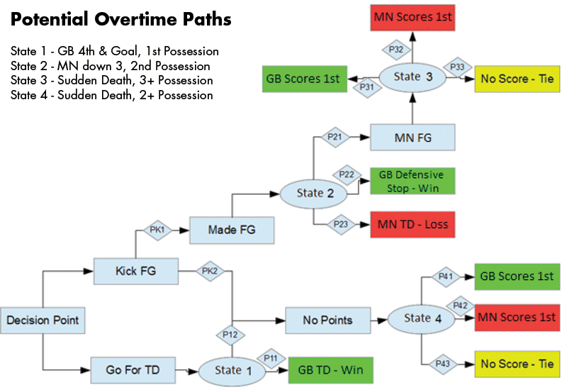
Figure 1. Overtime state map
The figure begins with the head coach’s decision. For our highlighted game, McCarthy opted to kick the field goal (FG) so we move to State 2, the point at which MN is down by three and must score at least a field goal. MN made a FG moving us to State 3, sudden-death overtime with GB receiving the kickoff, and only a fraction of the 15 minutes of overtime remaining. The outcome was a tie, which is highlighted in neutral yellow. If, however, McCarthy had opted to go for the touchdown (TD), we would move along the bottom of the figure. A TD result for State 1 means the game is over and GB wins. Failing to score results in a move to State 4. We are again in sudden death, but this is different from State 3 because now MN has the ball and must start deep within their own territory with more time on the clock.
Our first task was to decide which data to use to estimate the model probabilities. The data must match the situation in overtime as closely as possible and also be large enough to provide precise estimates. We utilized the NFL play-by-play data from the 2002 to the 2012 seasons, available on the AFA and NFL websites.
For the probabilities associated with State 1, we used all fourth-down-and-goal plays from the five-yard line and closer with at least five minutes to play in the half. A logistic regression model was fit to estimate the probability of a TD when attempted from each yard line. We also considered various measures of team strength, but surprisingly, only a binary proxy of a team’s ability to convert on fourth down was found helpful.
For the probabilities of State 2, we could consider all drives where a team receives a kickoff while down by three points, but that wouldn’t capture the do-or-die psychology of overtime. Instead, we first limited ourselves to the last drive of a game, where the team with the ball was down by three points and time did not run out mid-drive. These data were acceptable because the outcomes are identical to the part of overtime we need to model. Unfortunately there really wasn’t enough data to feel confident with the estimates. Thus, we opened it up to include the last two drives, which made a lot of sense for those games where a turnover is followed by the other team running out the clock. In the end, we also considered the last three and last four drives of the game before we felt we had enough data. Including all these drives begs the question: Did we lose the do-or-die sense of urgency we set out to get in the first place? Well, in all these drives, there was only a single punt. Teams were far more likely to turn the ball over on downs. Additionally, the probabilities were reasonably consistent across the different sets of data.
State 3 is sudden-death overtime but with less clock, since two FG drives have already occurred. There have been sufficient overtime games under the old sudden-death rules to estimate the probabilities for our situation. We estimated the average field-goal drive that begins with a kickoff return to be about five minutes in length. Two such drives should leave, on average, five minutes for sudden death. GB took over with 3:49 left to play, making five minutes seem like a reasonable cutoff value. So for our purposes, we use the old overtime data as if GB were receiving the opening kickoff and then see who scores first. If a score takes longer than five minutes, we call it a tie.
For the probabilities of State 4, we need to consider what happens when a team is pinned deep in their own territory. Which team is more likely to score first and how quickly? To answer this, we began by gathering all drives that started within the offense’s own five yard line. We then followed the ensuing drives for the next 10 minutes to see who scored first. If neither team scored within that time, we called it a tie. To account for the yard line, we utilized a multinomial logistic regression model to estimate probabilities for a win, loss, or tie.
So now that we have estimates of the model probabilities, we can estimate the probability of a win, loss, and tie for any yard line. Table 1 summarizes these results. In addition to yard line, it is also broken down based on a team’s ability to convert fourth downs.
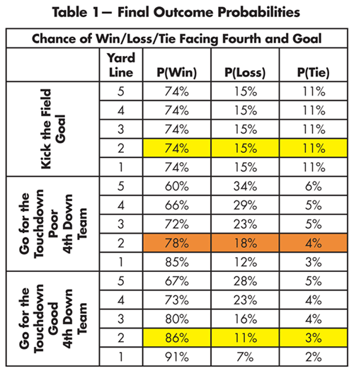
Table 1—Final Outcome Probabilities
Everything is from the perspective of GB. As an example, consider the highlighted orange row. This represents the probabilities for a team that isn’t particularly good at converting fourth downs and is facing fourth and goal from the two-yard line. If the team goes for the TD, it has a 78% chance of winning, an 18% chance of losing, and a 4% chance of tying. If the same team instead chooses to kick the FG (yellow highlighted row), there is a slight decrease in the probability of a win, and the probability of a tie is almost tripled.
So what does this table tell us about Coach McCarthy’s decision? That year, GB was very good at converting fourth downs. Had he gone for the TD, the model estimates that the probability of a win was 12% higher (86%) going for the TD compared to kicking the FG (74%). Also, the probability of a loss was 4% lower (11%) going for a TD compared to kicking a FG (15%). Clearly McCarthy made the wrong decision. Or did he? Yes, GB was very good at converting fourth downs, but most of those attempts involved Rodgers at quarterback. If GB is not a very good fourth-down converting team with Flynn, then we’re back to comparing the yellow- and orange-highlighted rows. These rows are quite comparable, with a slightly smaller probability of a loss when kicking a FG. Perhaps McCarthy was making the decision in terms of not losing. It turned out that GB won the NFC North Division by half a game, thanks to that tie. Had they lost, they would not have made the playoffs.
We worked really hard to extract data that matched the psychology of overtime from all available play-by-play data. We had to do this because there is not enough data that exactly matches the conditions. Thus, these probabilities are the result of our interpretation of overtime psychology. In addition, these probabilities are long-term averages using results across teams and years. Football coaches are paid to make these tough in-game decisions and may consider other factors that we could not extract from play-by-play data. Thus, providing a coach with this long-run information can be helpful as it brings some objectivity into the decisionmaking process.
From our results, we should expect more ties using this new overtime format. When the first team to possess the ball opts for a FG, there is about a one in nine chance of a tie. So should a team always go for the TD? Our model points to a cut-off at which the FG is the better choice. It depends somewhat on the team’s fourth-down conversion ability, but it’s around the three-yard line. This is a bit closer than what Burke found and a lot closer to the goal line than many might think.
Further Reading
Jones, Chris. 2010. A look at overtime in the NFL. Joint Policy Board for Mathematics (PDF download).
About the Authors
Bruce A. Craig is professor of statistics and director of the Statistical Consulting Service (SCS) at Purdue University. He received his MS and PhD in statistics from the University of Wisconsin-Madison. His research interests focus on the development of novel statistical methodology to address problems in a variety of research areas, including diagnostic testing, population dynamics, statistical genetics, and sports. He is an elected fellow of the American Statistical Association and was chair of its section on statistical consulting in 2009.
Zachary Hass is a PhD candidate in the department of statistics at Purdue University. He received his BA in statistics and economics in 2011 from Case Western Reserve University, where he also played for the football team. He currently works as a research assistant for the School of Nursing and as a game-day statistician for the athletic department at Purdue. Current research includes applications in animal science, health care, and sports.
Sean McCabe is a first-year PhD student in biostatistics at the University of North Carolina at Chapel Hill. He earned his bachelor’s degree in mathematics and statistics with a minor in computer science at Purdue University in 2014. His interests include statistical genetics and its applications in cancer research.

A Statistician Reads the Sports Pages takes a statistical look at sports. If you are interested in submitting an article, please contact Shane Jensen, column editor, at stjensen@wharton.upenn.edu.


