
A Simple Fix for Gerrymandering?
With the 2020 census results now in hand, election districts throughout the USA will have to be redrawn. There is fear that the process will be marred by partisan gerrymandering, meaning mischief by a state’s dominant political party to ensure that it wins more seats in future elections than are justified by its share of the popular vote. The U.S. Supreme Court considered the issue in both 2018 and 2019, and concluded that partisan gerrymandering was lamentable but not unconstitutional. The court noted, however, that citizens could take redistricting out of the hands of state legislatures in favor of commissions staffed by neutral professionals.
Indeed, voters in several states have approved the formation of such commissions—but such bodies might be more successful in theory than in practice. California took the lead in this regard when it created the California Citizens Redistricting Commission to set the boundaries of election districts. Yet in all nine California elections from 2014 to 2018, for State Assembly, State Senate, and U.S. House of Representatives, the share of seats won by Democrats exceeded their statewide vote share, by an average of 9.4 percentage points.
There is another way to reduce the discrepancy between a political party’s statewide share of votes and its share of seats in Congress or the state legislature. The proposed remedy is simple and might easily seem simplistic. It would focus not on changing the boundaries between election districts but on how the outcomes within these districts are processed. By its very construction, it would create equality between statewide vote shares and statewide seat shares. In doing so, it would introduce some new problems, but empirical evidence indicates that these problems are smaller than might be feared.
On Wisconsin
To illustrate the approach, turn to the 2012 Wisconsin election for the state assembly, which was at the heart of a gerrymandering case that the Supreme Court considered in 2018. In that election, Republicans won in 60 of the 99 assembly seats, even though they only received 48.6% of the combined votes for Republicans and Democrats. (Third-party vote totals were negligible.). Democrats won the other 39 seats.
Suppose that, mirroring the statewide vote split of 51.4% to 48.6%, Democrats were declared the winners in 51 of the 99 districts (i.e., 51.4% of 99). These districts would consist of the 39 that they won outright plus the 12 additional districts in which they were the closest runners-up. The remaining 48 districts would be allotted to the Republicans who won there.
By definition, this scheme would match Republican representation in the Wisconsin assembly with the Republican share of the statewide vote. It does so, however, by reversing the “first past the post” outcomes in 12 districts that the Republicans won. That circumstance is not ideal, but one could argue that it is the “lesser of two evils.”
More specifically, the Wisconsin Republicans won 60.6% of the Assembly seats in 2012. A total of 2.66 million two-party votes were cast in the assembly races and, ideally, 60.6% of the seats would correspond to 60.6% of the votes or 1.61 million votes. Yet Republicans only amassed 1.28 million votes statewide. If one believes that 1.61 million votes are needed to “deserve” 61 seats, the Republicans were in some sense credited with 330,000 votes (1.61 million minus 1.28 million) that actually went to Democrats. Put another way, 330,000 Wisconsin voters in some sense had their votes “reversed” and assigned to the other party (“statewide reversals”).
This “statewide-match” procedure would obviously cause Republican reversals in Wisconsin at the local level; namely, in those 12 districts where the Democratic runner-up took the assembly seat, even though the Republican got more votes, but such local reversals would be relatively rare. Typical of these outcomes is District 50, in which the Republican candidate got 12,842 votes in 2012 and the Democrat received 11,945. To actually win that district, the Democrat would have needed just over half of the 24,787 votes cast, which works out to 12,394. Thus, declaring the Democrat the winner in that district is tantamount to reversing 449 Republican votes (12,394 minus 11,945).
Over the 12 districts in which Wisconsin Democrats came closest to winning but lost, they would have been victorious had they received a total of 7,711 more votes. In other words, countermanding the 330,000 statewide vote reversals tied to alleged gerrymandering would have required 7,711 reversals at the local level (local reversals). Local reversals and statewide reversals are not totally equivalent but, because 7,711 is only about 2% of 330,000, the benefits of statewide match in this Wisconsin election might seem to substantially exceed its drawbacks.
This example might be interesting, but it raises several questions. Is this 2% ratio at all typical of recent elections or is it a statistical fluke? What about the 25 election districts out of 99 in Wisconsin in which one party offered no candidate, assuming that a loss was a foregone conclusion? (Such forfeitures would hardly persist if a party’s success were tied to its statewide vote share.) And isn’t it intrinsically unfair to deprive a legislative seat to the winner of a local election?
Discussing these issues involves formalizing this analysis.
The Statewide Match Approach
Central to the process outlined for Wisconsin—referred to henceforth as statewide-match—is the calculation of effective vote reversals, both initially at the statewide level and locally when runners-up are declared the winners.
When the focus is on a two-party two-candidate race (parties A and B), and it is assumed that party A is the one whose share of seats won in an election exceeds its vote share (called the advantaged party), definitions are:
- N = total votes cast statewide in the election
- Q = number of legislative seats up for election
- SA = proportion of seats won by Party A under current rules
- VA = proportion of votes won by Party A statewide (VA < SA)
Then, NSA is the number of votes that Party A would have needed for its seat share and vote share to be the same. Under statewide match, NSA is treated as the level of support that is required to justify getting QSA seats.
If quantity R1 is the number of votes for Party B that were effectively reversed and assigned to Party A, if the latter’s seat share were matched to its vote share, then R1 follows:
R1 = NSA – NVA
Under statewide-match, Party A’s number of seats would be reduced to QVA while Party B’s seats would increase from Q(1 – SA) to Q(1 – VA). This would be achieved by treating Party B as the winner in:
- All the election districts it actually won and
- Some election districts that Party A won but in which Party B is declared the winner.
DAB, the number of districts in the latter category is Party B’s number of victories had its seat share equaled Q(1 – VA) minus the number it actually won (in the Wisconsin example, that number was 61 – 49 = 12). The specific districts reassigned to Party B would be those DAB districts in which it was the closest runner-up to Party A, in terms of number of votes received.
If τAB is Party A’s lead in total votes over the DAB districts, then Party B would have carried these districts had it received as few as τAB / 2 additional votes. This would happen if Party B’s gain in each individual district was half of Party A’s margin of victory. (Technically, it would need ever-so-slightly more than half of Party A’s victory margin.) Therefore, R2, the total number of votes that are effectively reversed at the local level under statewide match, follows:
R2 = τAB / 2
The ratio R2 / R1 expresses local votes “reversed” under statewide match as a proportion of statewide votes reversed under current arrangements. The quantity RR = 100(1 – R2 / R1) is the percentage reduction in vote reversals in moving from the status quo to statewide match.
No Unopposed Candidates
A prerequisite to exploring statewide match with actual election data requires dealing with single-candidate races, which are far from scarce in many U.S. states. As noted, such “races” would presumably disappear if each party were trying to maximize its share of the statewide popular vote. McGee and Stephanopoulos worried about single-candidate elections in their own research about elections, and developed extensive procedures to estimate how voting outcomes would change if no candidates ran unopposed. Table 1 reports their estimates of the average effect over the elections they studied.
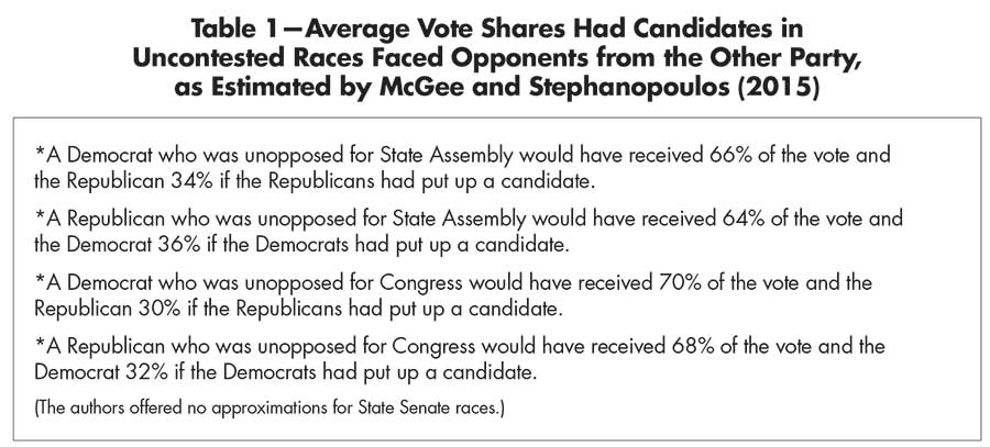
Table 1—Average Vote Shares Had Candidates in Uncontested Races Faced Opponents from the Other Party, as Estimated by McGee and Stephanopoulos (2015)
McGee and Stephanopoulos found variations in these averages in individual races, but these are treated here as point estimates in forthcoming calculations.
Data about single-candidate races can be processed in three ways—as if:
1. The results actually occurred.
2. The existing votes for the lone candidate were split with a new opponent of the other party, according to the relevant MS approximation in Table 1.
3. The existing candidate’s vote tally remains the same, but the new opponent gets enough additional votes to achieve the vote-share specified by the relevant McGee and Stephanopoulos approximation.
For example, in a State Assembly race with only a Democratic candidate who got X votes, that candidate would get .66X votes under Alternative II, while the new Republican would get .34X. Under Alterative III, the Democrat would still get X votes, but the Republican would get (34/66)X, yielding a Republican vote share of 34%. (Alternative III could arise because Republican voters might refuse to mark their ballots in races with unopposed Democrats.)
Some Empirical Findings
This analysis focuses on three recent election years—2014, 2016, and 2018—and three kinds of elections: for Congress, State Senate, and State Assembly. The years differ somewhat because only 2016 saw a presidential election, while 2014 was a strong year for Republicans and 2018 was strong for Democrats. The issue is whether the effectiveness of statewide match is robust across such variations.
Table 2 presents results for Congress, State Senate, and State Assembly in 2018. They concern all states that had at least six members of the U.S. House of Representatives (smaller states, seven of which have only a single Congressional district, are treated as less appropriate candidates for statewide match). Averaged across the states, vote reversals dropped by approximately 96% in Assembly races, 97% in state Senate races, and 95% in Congressional races. The decline was lowest in Congressional races, which is unsurprising because election districts for Congress are typically far less numerous than districts for statewide offices, meaning that there is a lesser chance of finding districts where the disadvantaged party’s candidates were close runners-up. Indeed, it is striking that the congressional results are as close as they are to the statewide ones.
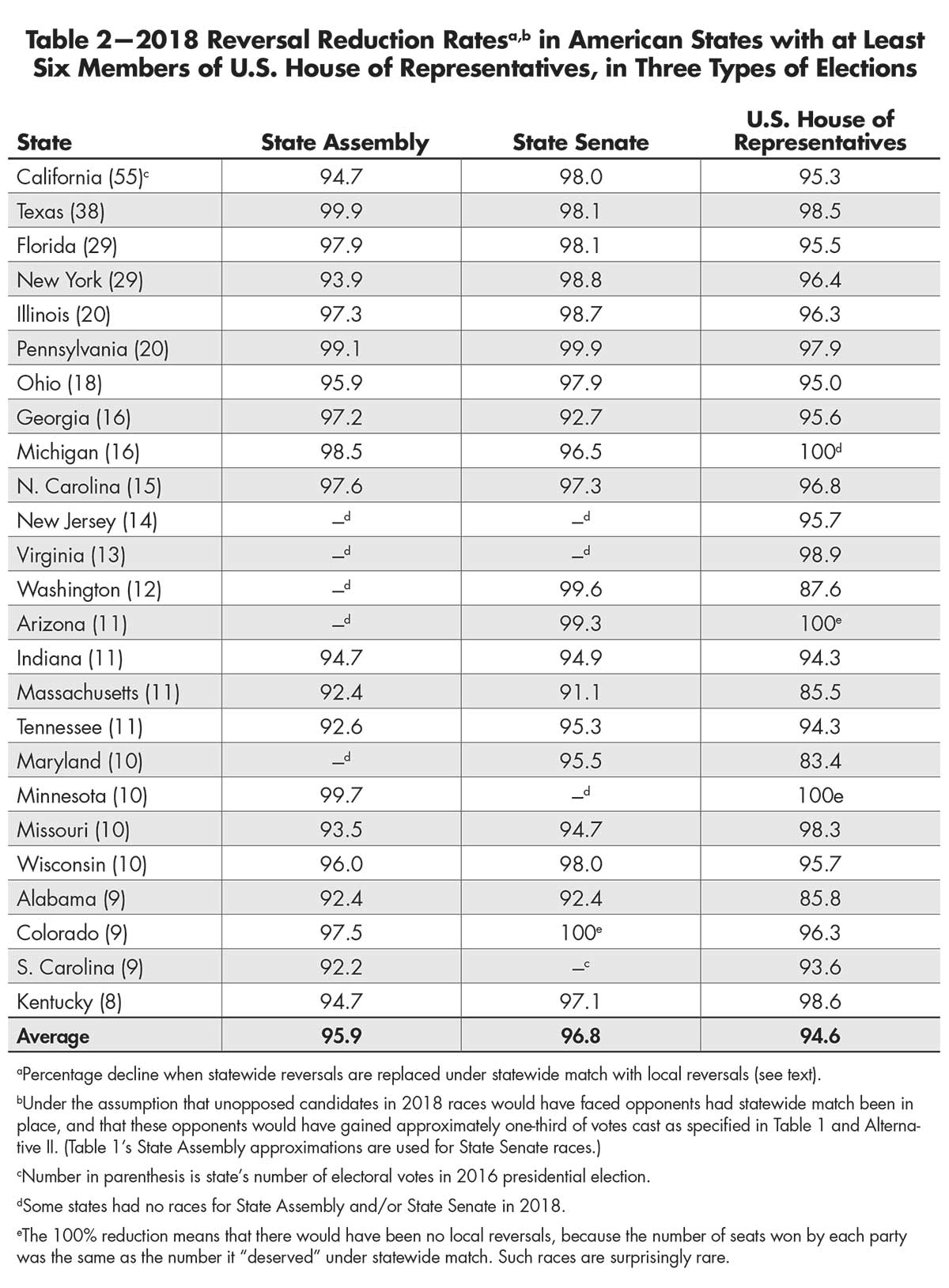
Table 2—2018 Reversal Reduction Ratesa,b in American States with at Least Six Members of U.S. House of Representatives, in Three Types of Elections
Table 3 reports on the elections of 2014 and 2016. The overall results are very similar to those for 2018; the main difference is that the reversal-reduction rate for Congressional races fell slightly. That the results for 2014, 2016, and 2018 were so close together implies that reversal reductions under statewide match are essentially the same, regardless of turnout or of which party was dominant in the election.

Table 3—Average Reversal Reduction Rates Under Statewide Match for Three Kinds of Elections in Three Years, Among States With at Least Six Members of the U.S. House of Representatives
Tables 2 and 3 are based on one of the three methods considered for dealing with unopposed candidates; namely, the one that split existing votes between the two parties and gave approximately two thirds to the party that fielded a candidate. Table 4 presents the corresponding calculations under the other two approaches. The mean reduction rates were essentially the same for all three methods, which suggests that uncertainty about how statewide match would affect uncontested races has little effect on the decline in reversals under that policy.
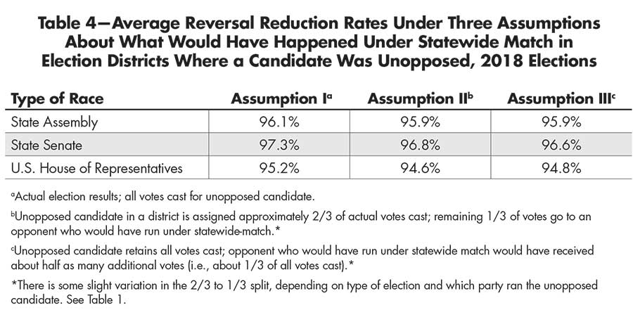
Table 4—Average Reversal Reduction Rates Under Three Assumptions About What Would Have Happened Under Statewide Match in Election Districts Where a Candidate Was Unopposed, 2018 Elections
These outcomes imply that the sharp reduction in reversals in the original Wisconsin example was not an aberration. In recent years, local reversals under statewide match are about a factor of 20 less numerous than statewide reversals under existing rules.
Why Statewide Match?
In summary, the case for a statewide match scheme is the following:
It Is Fairly Easy to Explain and, by its Very Nature, Ends the Disparity Between Statewide Vote and Seat Splits for the Two Major Parties, in both the State Legislature and the House of Representatives
Not only is that a desirable outcome in its own right, it all but eliminates the advantage of devising districts with bizarre shapes to further partisan advantage, and it eliminates lopsided outcomes no matter why they arose. This is important because large discrepancies between vote shares and seat shares can arise in states that have not recently been accused of gerrymandering.
It Would Reflect What Happened in This Election, Not What Happened in Previous Elections
Attempts to create “fair” districting typically use outcomes of past elections as guides to setting district boundaries, but changes in voter composition and preference can limit the power of historical results to predict future outcomes. Because the proposal here does not treat “the past as prologue,” it avoids the hazards of doing so.
It Is Easy to Implement, as Soon as Votes Are Counted
District-by-district vote counts are known the day after the polls close (barring delays tied to absentee ballots). Thus, the number of seats won by each party are at hand, along with the identity of the districts awarded to each party under the statewide match policy.
Implementation of the Policy is Not Contingent on What Other States Do
Proposals to replace the Electoral College with (say) a popular vote often depend on the coordinated activities of various states. That issue does not arise here: If Pennsylvania wishes to implement statewide match, the fact that Colorado opts otherwise poses no problems.
Every Vote Counts Under the Policy
Even those voters who suffer local reversals—meaning that their candidates get the most votes but other candidates get seated under statewide match—are not fully deprived of influence: They affect the statewide vote split between the parties in favor of their preferred party.
Local Vote Reversals Are Rare Compared to Statewide Vote Reversals that the Policy Eliminates
The empirical evidence presented here establishes this point, with reversals down about 95% on average. The data show that, typically, there are many districts in which the winner gets only slightly more votes that the loser. Thus, occasionally awarding a seat to the runner-up involves reversing only a small fraction of the votes cast.
Yet, the proposal has an obvious disadvantage: It does not seem ideal when the winner in a local district is denied the seat they won. First-past-the-post elections are traditional, and they accord with the sense of fair play, but deviations already exist. In Georgia in 2020, the candidate who got the most votes in a Senate election (Perdue) was not chosen because he got fewer than 50% of votes cast (he was defeated in the subsequent runoff race). And increasingly in elections with several candidates, voters can accompany their first-choice listing with second and later choices.
In such elections, the candidate with the most first-choice votes can lose to someone with greater strength in later-choice listings. Such ranked-choice voting is already in place in about 20 U.S. cities; in a 2019 referendum, voters in Maine instituted the policy for future elections. New York City’s 2021 primary election for mayor used ranked-choice voting, and there was much speculation that the first-place finisher would lose. (Multiple candidates are more common in primary elections than in final ones.)
The German Parliament Example
The statewide-match proposal bears some similarity to the method used to elect members of the German Parliament (the Bundestag). The country is divided into 299 election districts, each of which chooses one member of Parliament under the first-past-the-post rule. But each voter also chooses one party, and 299 additional members are chosen “at large,” so each party’s total representation in Parliament equals its share of the national vote by party. For example, if a given party wins 24 seats out of 299 in the direct elections but 10% of citizens voted for that party, then it would get 36 of the at-large members and would gain (24 + 36) / 599 ≈10% of parliamentary seats.
This selection method avoids the local reversals that would arise under statewide match, but it means that half of those elected to Parliament were not on the ballot. Arguably, it is more problematic to have a majority of parliamentarians without ties to specific communities than a few legislators who got slightly below half the vote in their home districts. Furthermore, Balinski also proposed equating a party’s statewide seat share to its vote share, although he would have candidates for each party “compete” for its seats based on absolute numbers of votes. He did not perform any data analysis on his proposal.
Final Remarks
This discussion may seem hopelessly impractical, because no legislature would ever forego its power to set election districts in favor of statewide match. This is probably true, but the legislature might not have a choice: Voters could establish the system by referendum. That is the mechanism by which neutral redistricting commissions were created in several states, most recently in Virginia in 2020. As the California experience suggests, however, these commissions might struggle to align legislative seat shares by party with statewide vote shares.
This is not to say that neutral redistricting is not valuable. It would eliminate districts with strange shapes devised to benefit one political party, which are weird concoctions both geographically and politically—and the combination of neutral redistricting and statewide match might achieve the best of both worlds. When redistricting yields parity between statewide seat shares and statewide vote shares, statewide match would stay in the background and offer at most some fine-tuning. When election results differ from those anticipated by the commissions, though, statewide match offers an automatic mechanism for bridging the gap.
The question is whether election procedures that include statewide match can yield fairer outcomes than those without it. This article makes a case that the answer is yes.
Further Reading
Balinski, M. 2008. Fair Majority Voting (Or How to Eliminate Gerrymandering). American Mathematical Monthly 115(2), 97–113.
FairVote. Retrieved in 2020. Open Ticket Voting.
FairVote. 2013. Independent Districting and Districts Plus: A Powerful Reform Combination.
Gelman, Andrew, and King, Gary. 1994. Enhancing Democracy Through Legislative Redistricting. American Political Science Review 88, 541–559.
Stephanopoulos, Nicholas, and McGhee, Eric. 2015. Partisan Gerrymandering and the Efficiency Gap. University of Chicago Law Review 82, 831–900.
About the Authors
Arnold Barnett is the George Eastman Professor of Management Science and professor of statistics in the Sloan School of Management of the Massachusetts Institute of Technology in Cambridge, MA.
Pengchen Han and Gege Zhang are students in the master’s of business analytics program in the Sloan School of Management of the Massachusetts Institute of Technology in Cambridge, MA.


