
A Modification to Pull the Goalie that Takes the State of Play into Account: Coach Markov Returns

A recent paper by Asness and Brown (2018) reignited interest (the paper has about 34,000 downloads on SSRN and is ranked 40 on the website) in the “Pulling the Goalie” strategy used by coaches in ice hockey games when their teams are down. The Asness-Brown (AB) model used dynamic programming to cleverly update the answer to a perennial problem that this lead author tackled back in 2001.
The model was widely heralded as a breakthrough and the result was consistent with the paper by Zaman (2001). Asness and Brown acknowledged that having a stateful model might improve the decision-making power of the AB model; specifically, that knowing if the puck is in the offensive zone, neutral zone, or defensive zone would vary their recommendation. This paper uses that same approach, while making some modifications that take into the account where the puck is located initially. It also assumes that the coach has to live with the decision until the next face-off.
Our results find that the optimal time for pulling the goalie, if the team is down by one goal and has a face-off in the offensive zone, is a full 3 minutes earlier. The two takeaways we would add to the brilliant AB model have a wide variety of practical uses for understanding risk.
First, insights about state matter. A piece of information about your advantage or the state of your game markedly changes the decision. It protects your risky decision. If you have a low probability bet, you have to make it with the downside in view and look for an insight that tells you when you can take more risk. Second, insights are fleeting. Their half-life is short. Even though the state is one way now, it will change in a very short while, and you will lose the insight advantage.
Model by Asness and Brown
AB is a straightforward dynamic programming model that uses five inputs: the probability of scoring goals with a goalie in place, goalie pulled for an extra attacker, goalie in place but the other team has pulled their goalie for an extra attacker, goal differential, and time remaining in the game.
The time remaining in the game is broken up into 10-second intervals, and the probabilities of scoring with the goalie in place and not in place are estimated using data from the 2015–16 NHL season. When the goalie is not pulled and both teams have even strength, the analysis in Asness and Brown gives a 0.65% chance of scoring in each 10-second interval. When one team has pulled the goalie, the scoring rate becomes 1.97% per 10-second interval for the team with the sixth attacker, and 4.3% for the team that keeps its goalie.
The goal differential is represented by S, and is positive if the team in question is leading, zero if the game is tied, and negative if they are trailing. In hockey, a team gets 2 points for a win, 1 for a loss in overtime, and 0 for a loss in regulation time. Asness and Brown use 1.5 points for how much a tie is worth at the end of regulation play.
To solve for the optimal strategy, they first define the expected point function of never pulling the goalie in any situation, given as EPNP (score differential, time remaining). This is called the “Tikhonov” option and is:
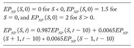
If the goalie is not pulled, each team has a 0.65% chance of scoring in each 10-second period. This means that a team has a 0.65% chance of scoring, which increases the score deferential (S + 1), or a 0.65% chance of being scored on, decreasing the score differential (S – 1). Since these probabilities are mutually exclusive, the chance that the score differential remains the same (S), which is given as 1 – 0.0065 – 0.0065 = 0.987, can be computed. Working backward from 10 seconds left makes it possible to compute EPNP (S, t) for all S and t.
The expected point function if you pull now and act optimally thereafter, EPPO(S, t), and if you don’t pull now and act optimally thereafter, EPNO(S, t), are defined similarly as follows:
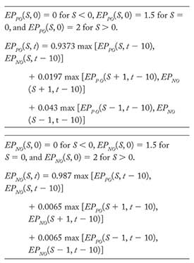
Again, all EPPO and EPNO values can be found by working back in 10-second intervals from the end of the game. This is the AB model. The optimal time to pull the goalie is right when EPNO < EPPO (see Asness and Brown (2018) for more details about the AB model). We take the result that the AB model gives 370 seconds as the optimal time to pull the goalie.
Our Modification
We make two additions to the AB model.
Modification 1: What zone is the puck in?
The AB model does not take the state of the game into account. We take inspiration from Zaman (2001) and incorporate the state of the game into the dynamic programming model. Without loss of generality with respect to team A, the ice hockey rink is divided into three zones: neutral, offensive, and defensive. We assume that the coach only knows that the puck will be in each zone respectively for the first 10-second block. After that, he has no idea where the puck will be, and the model reverts back to the stateless AB model.
In the offensive zone, there is 0 probability of Team A being scored on by Team B. Hence, we modify the probabilities in the AB model using Bayes’ theorem. Under the Tikhonov strategy, where the goalie is never pulled, the new probability of the score differential S remaining the same is
![]()
This gives the probability of Team A scoring and increasing S to S + 1 to be 1 – 0.99346 = 0.00654. Similarly, when the goalie is pulled, the probability of S remaining the same is
![]()
This gives the probability of S becoming S + 1 to be 1 – 0.9794 = 0.0206.
In the neutral zone, we assume that this is the state of the AB model, and the probabilities remain the same. Under the Tikhonov strategy, the probability of S changing to S – 1 is 0.0065, S remaining as S given by 0.987, and S to S + 1 is given by 0.0065. When the goalie is pulled, these probabilities change to 0.043, 0.9373, and 0.0197, respectively.
In the defensive zone, we assume that there is 0 probability of Team A scoring on Team B. Again, we update the probabilities using Bayes’ theorem. Under Tikhonov, the probability of S not changing is
![]()
and the probability of S going to S – 1 is 1 – 0.99346 = 0.00654. When the goalie is pulled, the probabilities are
![]()
and 1 – 0.9561 = 0.0439, respectively.
Modification 2: Inability to put goalie back if state changes until next face-off
The second modification that we made to the AB model is to suggest that once a coach has taken a decision, he cannot revert to putting the goalie back in instantaneously if the state (puck location) changes. This is a pragmatic and realistic assumption since it is inadvisable to put a goalie back until play is stopped and state has reverted. To model this, we incorporate a time freeze to account for the next stoppage in play. We estimate the arrival time of face-offs in NHL games using data from the 2017–18 NHL season, which comes to an average of one face-off per 60 seconds.
Given this, we make the assumption that for those six 10-second intervals, even though the coach has decided to put the goalie back into the game, the probabilities remain at the AB model’s pulled goalie probabilities. It is as though the goalie is still pulled, since the coach has to live with the decision.
Results
When a team is down by one goal, we should find the crossover points for the neutral zone, offensive zone, and defensive zone cases, keeping an eye out for how they differ in their advice. We calculate all of our results for a score differential of S = −1.
First, we have to reprogram the expected point functions to incorporate a time freeze whenever the goalie is pulled and the coach wants to put the goalie back in. We can compare the results from the AB model and our model with a freeze (not including starting state). Our expected point value advantage over never pulling with a freeze is shown in Figure 1.
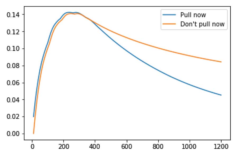
Figure 1. Expected point value advantage over never pulling with a 60s freeze. The crossover point occurs at 340 seconds.
Figure 1 shows the expected point value advantage over never pulling with a time freeze of 60 seconds, with the crossover time at 340 seconds, which means pulling the goalie at 330 seconds. This means that at 340 seconds, not pulling gives a higher payoff. Hence, we should pull the goalie at 330 seconds. Our results are similar to the AB model because the time freeze does not affect the stateless result much if the coach keeps the goalie pulled and never puts him back into the game.
If we assume that the coach can put the goalie back in faster than 60 seconds, the shorter time freeze results in an even smaller difference, which explains why with only a 20-second time freeze, we get almost the same results as the AB model.1
Next, calculate the expected point value advantage over never pulling with freeze starting from the offensive zone, neutral zone, and defensive zone, respectively.
Starting from the offensive zone, Figure 2 shows that with a freeze of 60 seconds, the crossover time is at 560 seconds, giving the optimal time to pull the goalie at 550 seconds. If we assume that the coach can put the goalie back in 20 seconds, the crossover time extends dramatically to 910 seconds, which means that the optimal time to pull the goalie is at 900 seconds.
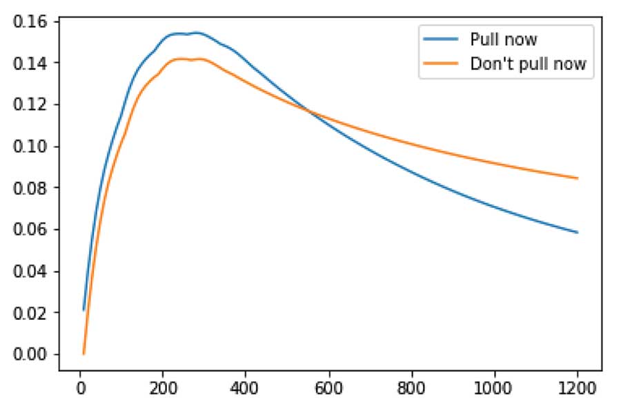
Figure 2. Expected point value advantage over never pulling with a 60-second freeze starting from the offensive zone. The crossover point occurs at 560 seconds.
Starting from the neutral zone, the expected point value advantage over never pulling with a 60-second freeze is exactly identical to Figure 1. This is because Figure 1 is the stateless model, which we assume starts from the neutral zone. Hence, the crossover times and pulling times are exactly the same here.
Finally, starting from the defensive zone, the crossover point occurs at 20 seconds and the optimal time to pull the goalie is at 10 seconds.
Our results make sense intuitively. When we are down one and the puck is in the offensive zone, we should definitely pull the goalie at a much-earlier time compared to when the puck is in the neutral or defensive zone, to take advantage having the puck and gaining an advantage to try to score.
Our model has an advantage over the AB model in that it gives us a strategy that coaches can use dynamically. Instead of keeping the goalie pulled as in the AB model, the coach now has a strategy that depends on the time remaining and the zone that the puck is in. The coach should follow the following strategy given in Table 1.
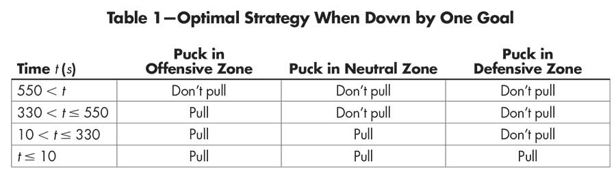
Table 1—Optimal Strategy When Down by One Goal
That is, the coach pulls and puts back the goalie according to the time left in the game and position of the puck.
We can also use our model for when the team is down by two goals. The optimal time to pull the goalie now increases to 1,180 seconds, 760 seconds, and 20 seconds, starting from the offensive, neutral, and defensive zone, respectively. Once again, our result of 760 seconds in the neutral zone is similar to the 780 seconds obtained by the AB model. A coach facing a two-goal deficit should amend the times accordingly in Table 1, and revert back to the original times if they improve the deficit to one goal.
Finally, it is possible for a coach to calibrate our model according to the team’s relative ability. This can be done by using team-specific data. For example, the probability of scoring goals while at full strength for a particular team can be estimated by taking the number of such goals scored by the team, divided by the time played at that strength by the team. Similar calculations can be done for the probabilities of being scored on at full strength and when the goalie is pulled. The analysis can then be done again using the same procedure as outlined before.
Why Don’t Coaches Pull Earlier?
Given our optimal strategy, it seems that coaches should pull their goalies much earlier when they are a goal down, depending on the location of the puck. This aligns with other models that show that coaches should pull the goalie much earlier than is actually observed in a game. Why, then, aren’t coaches taking this risk and, as Malcolm Gladwell pointed out, being disagreeable? Our model gives what we think is a reasonable explanation.
If the time is between 330 seconds and less than or equals to 550 seconds, the coach should pull the goalie when the puck is in the offensive zone, and put the goalie back when the puck is in the neutral or defensive zone. In a hockey game, the puck is traveling very quickly between these three zones all the time, so state insight is fleeting. Coaches need air cover. They need an explanation that works with the fans. Only when the coach can justify that, because he has the advantage of an offensive zone face-off and the risk of being scored upon drops to zero, would he have permission to be bolder. What mitigates the decision is that if he does not get the equalizing goal, he has to live with his decision until the play stops.
Hence, even though it is optimal for the coach to adjust his strategy according to the location of the puck, it may be that these changes happen too quickly for it to be effective. Effectively, “Pull the Goalie” is about making unpopular risky decisions that require courage. The nuances we uncovered about state should color perception of all risky decisions and how it is perceived. Gladwell’s famous question “Do you run to get help when a robber is in your home with you and your children?” is made easier if you know that your children are safe for a while, but only if you hurry.
In management, look to discrete decisions to find “Pull the Goalie”-type risks, usually when a company or a leader is in a crisis or under pressure to perform a turnaround. Some examples could be a CEO at the end of a middling tenure acquiring a blockchain startup, an under-performing portfolio manager investing in riskier assets to rescue a bad year, or a struggling studio executive green-lighting an arthouse feature from a first-time screenwriter. Our model suggests that, if the decision-maker obtains a temporary insight that reduces downside (e.g., Meryl Streep has agreed to play the lead), it can be used as justification to de-risk the potentially sour taste of entering into a project that might have seemed desperate.
De-risk risky decisions with bits of certainty.
A keen insight about the state of the system (e.g., a short-lived zero risk of a major downside) may it possible to temporarily take a “Pull the Goalie” type of risk. If the switching costs or freeze time is low or zero, then someone can keep taking calculated risks strategically only with the benefit of being in an advantaged state.
Further Reading
Asness, Clifford S., and Brown, Aaron. 2018. Pulling the goalie: Hockey and investment implications.
Zaman, Zia. 2001. Coach Markov Pulls Goalie Poisson. CHANCE 14(2):31–35.
Footnote
1Our model with time freeze of 20 seconds suggests pulling at 380 seconds. The AB model gives 370 seconds.
About the Authors
Zia Zaman has spent 27 years as a corporate executive, most recently as chief innovation officer at LumenLab, MetLife. Much of his inspiration sprouted on the two campuses where he studied, Stanford and MIT, where he wrote about probability, traveling salespeople, small towns in Asia, parenting special needs children, “The Price Is Right,” innovation, and hockey.
Hong Ming Tan is a third-year PhD student at the Institute of Operations Research and Analytics, National University of Singapore. His research interests are in stochastic control, sports analytics, and revenue management.


