
The Mathematical Anatomy of the Gambler’s Fallacy

The gambler’s fallacy is one of the most deeply rooted irrational beliefs of the human mind. Some 200 years ago, the French mathematician and polymath Pierre-Simon de Laplace (1749–1827) assigned a prominent place to this fallacy among the various illusions common in estimating probabilities. In his classic Philosophical Essay on Probabilities, he recalled seeing men who, on the verge of becoming fathers and ardently desiring sons, learned with anxiety about the births of boys, believing that the more boys were born, the more likely their own child would be a girl. In the same essay, Laplace also recounted how people were eager to bet on a number in the French lottery that had not been drawn for a long time, believing that this number would be more likely than the others to be drawn in the next round.
Times change, people don’t. Not so long ago, a single number in the Italian state lottery held almost an entire nation in its spell. Number 53 eluded every draw for more than a year and a half. With each draw, more and more Italians believed that the magic number would surely emerge. It took 183 draws to end the “collective psychosis,” as it was called. Many people were left with heavy debts, some went bankrupt, and a few even committed suicide.
Not without reason is this belief known as the gambler’s fallacy. Its fallacious nature is best illustrated by the flip of a fair coin.
Imagine that you flip a coin and the coin lands heads-up four times in a row. On the next toss, it is hard to ignore that inner voice called intuition that assures you the coin will land tails-up. After all, the series of heads must come to an end. Otherwise, the coin would appear to favor one of its two possible outcomes and would no longer be fair.
This may seem like common sense to many people, but of course, it is not. A coin has no memory, so how can it compensate for previous outcomes? It cannot. Whatever the previous outcomes, the odds remain exactly the same. Clearly, our intuition is wrong.
And yet most of us are uncomfortable with runs of five or more heads or tails in a row. It is well known that, when asked to make up a random sequence of 100 coin tosses, people will as a rule avoid runs of five or more consecutive heads or tails. And why wouldn’t they? The probability of a series of five heads or tails in a row, as can be easily calculated, is only 1/16, so the probability of this happening is just over 6%—or so it seems. But once again, we are wrong.
People forget that this is only true if you flip a coin exactly five times. But in a series of 100 tosses, there are 96 starting points for a sequence of five. If you flip a coin 100 times, there are many opportunities to get five heads or five tails in a row. Clearly, the probability must be considerably larger, but how much? Counting all the favorable outcomes of 100 coin tosses would be a herculean task, because the total number of possible outcomes exceeds 1 million. Fortunately, there is another, more elegant way to find the probability we are looking for: a transition matrix (for the basics of this method, see, for instance, Tijms. 2021).
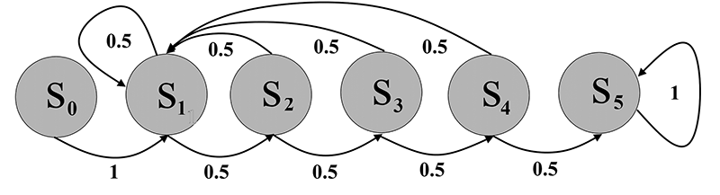
Figure 1. Transition diagram.
The Mathematics of Long Runs
To toss a series of five or more heads or tails in a row, the coin must pass through six consecutive states. Let’s call them s0, s1, s2, s3, s4, and s5. State s0 is the starting state: The coin has yet to be tossed. State s5 is the final state: You have tossed five or more heads or tails in a row. The other states—s1, s2, s3, and s4—are the intermediate ones in which you have tossed a sequence of, respectively, exactly one, two, three, or four consecutive heads or tails. The possible one-step transitions between these states can be represented in a transition diagram.
When you toss the coin for the first time (s0), you can clearly only advance to state s1 (either heads or tails), so Pr(s0 → s1) = 1. Other one-step transitions from state s0 are impossible and therefore have a probability of 0. Once you have arrived at state s5, you have reached your goal. Whatever the outcome of the next toss, you will remain in s5, so Pr(s5 → s5) = 1. That is why it is also referred to as the absorbing stat. All other transitions from state s5 have a probability of 0.
From each of the intermediate states si, you can, with equal probability, either move to si + 1 if you toss the same outcome as the previous one, or, if not, return to state s1, so Pr(si → si +1 ) = 0.5 and Pr(si → s1) = 0.5. Other transitions from state si have a probability of 0.
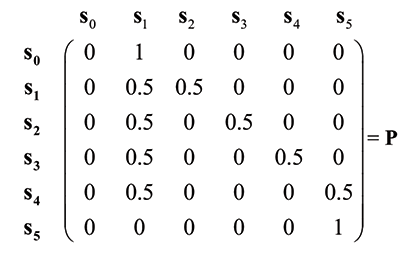
These probabilities can be arranged in the form of a matrix. The first row shows the probabilities for the one-step transitions from state s0 to states s0, …, s5, respectively. The second row shows the probabilities for the one-step transitions from state s1 to states s0, …, s5, respectively, and so on, up to state s5. Such matrices are appropriately called transition (probability) matrices. They were first used by the Russian mathematician Andrey Markov (1856–1922) and are therefore also known as Markov matrices. This is what the one-step transition matrix P looks like:
Since a transition matrix is square, it can be multiplied by itself. It is not difficult to see that if you multiply the matrix P by itself, you get a matrix, P2, whose elements are again the probabilities of going from one state to another, but this time in two tosses of a fair coin. In general, the elements of the n-fold product of matrix P with itself (Pm) are exactly the probabilities of going from one state to another state in n tosses of a fair coin. To find the probability of a run of five or more consecutive heads or tails in 100 tosses, we only have to calculate P100.
Multiplying matrices is a tedious and labor-intensive task, but fortunately, several online matrix calculators on the Internet (e.g., matrix.reshish.com) will do the work in no time. The probability we’re looking for is given by the last element in the first row of P100. It is 0.972. In other words, not a meager 6.25% but an amazing 97.2%! So, completely contrary to what people tend to think, it would be exceptional for a run of five or more heads or tails in a row not to occur.
Even longer runs have a more than 50% chance of occurring in 100 tosses. In the same way as above, the probability of a run of six or more heads or tails in a row can be calculated as 80.7%, and the probability of a run of seven or more heads or tails in a row is 54.2%. Even a run of eight or more heads or tails in a row still has a 31.5% probability of occurring. In short, flipping a fair coin is, in fact, characterized by long runs of the same outcome. But if these long runs of the same outcome are quite normal, then why is the gambler’s fallacy so compelling?
The Belief in the Law of Small Numbers
A basic law of probability says that the longer you keep flipping a fair coin, the smaller and smaller the difference tends to become between the average number of heads and the average number of tails—even though the overall difference between the number of heads and the number of tails tends to grow. In other words, the relative frequencies of heads and tails increasingly tend to reflect their equal probabilities. This law of probability is the well-known law of large numbers.
In a 1971 paper entitled “Belief in the Law of Small Numbers,” published in the Psychological Bulletin, two psychologists—the late Amos Tversky and Nobel Prize-winner Daniel Kahneman—wrote, “People’s intuitions about random sampling seem to satisfy the law of small numbers, which claims that the law of large numbers also applies to small numbers.” They called this the belief in the law of small numbers. Applying the law of large numbers to small numbers typically causes people to commit the gambler’s fallacy, because it requires compensating for runs of the same outcome. Tracing the source of this misguided belief might help with understanding why it is so easy to fall prey to the gambler’s fallacy.
The Representativeness Heuristic
Tversky and Kahneman themselves gave a now-widely accepted account. They explained the belief in the law of small numbers as a cognitive bias arising from the way human judgment works in situations of uncertainty. In uncertain situations, roughly two cognitive mechanisms are at work. An intuitive way of thinking (also known as system 1) and a more analytical way of thinking (also known as system 2). Kahneman (2012) refers to these as fast thinking and slow thinking, respectively. Solving a probability problem, for instance, falls into the category of slow thinking, at least for most people. Gambling typically falls into the category of fast thinking.
When we think fast, we do not put much effort into analyzing a problem. Instead, we use heuristics. These are a kind of built-in mental shortcuts to making quick judgments under uncertain conditions. According to Tversky and Kahneman, the belief in the law of small numbers has its roots in a heuristic they called the representativeness heuristic. How this heuristic works is best illustrated by an example, using a stereotype mentioned by Kahneman (2012) himself: that young men are more likely than elderly women to drive aggressively. This bias can be explained in the following way.
Let’s say that police records show that most cases of aggressive driving involve young men. Few offenders are elderly women. Intuitively, it can be inferred that aggressive driving is apparently representative of young men. Young men, we conclude, are more likely to drive aggressively than elderly women.
Concluding this, however, is actually mixing up two different conditional probabilities:
(1) If someone is driving aggressively, then that person is more likely to be a young man than an elderly woman.(fact)
(2) If someone is a young man, then they are more likely to drive aggressively than an elderly woman. (bias)
By construing (1) to mean that aggressive driving is representative of young men, we incorrectly arrive at (2)—incorrectly, of course, because the representativeness heuristic does not take into account the simple fact that far more young men than elderly women drive cars. This error is known as base rate neglect.
Accordingly, the representativeness heuristic can lead to cognitive bias, and since heuristics are built into our brains, eradicating these cognitive biases can prove very difficult. If it can be shown that the belief in the law of small numbers has its roots in the same representativeness heuristic, that would go a long way toward explaining why the gambler’s fallacy is so powerful.
Insensitivity to Sample Size
In their 1971 article, Tversky and Kahneman wrote, “We submit that people view a sample drawn randomly from a population as highly representative, that is, similar to the population in all essential characteristics.” They claimed that people do so without regard to sample size, calling this bias insensitivity to sample size.
Again, the representativeness heuristic is to blame. Tversky and Kahneman were not very explicit about how the heuristic works in this case, but we can show that once again, two conditional probabilities are being mixed up:
(1) If a population has a salient characteristic A, then a random sample from this population is likely to have the same characteristic A. (fact)
(2) If a random sample has a salient characteristic A, then the population is likely to have this characteristic A as well. (bias)
From (1), intuition concludes that random samples are representative of their population. Hence, we incorrectly arrive at the inverse probability (2). This time, the representativeness heuristic ignores that small samples are much more susceptible to chance variation than large samples are and therefore need not be representative at all. For example, one crime more or one crime less in a year has a much greater impact on the crime rate in a small town than in a large city. Such chance variations in the crime rate of a small town are, of course, not representative of the overall level of criminal activity at all.
The Gambler’s Fallacy
But how does the gambler’s fallacy fit into this? Tversky and Kahneman argued that insensitivity to sample size also manifests itself in generating random sequences, as, for instance, in flipping a coin: “Subjects act as if every segment of the random sequence must reflect the true proportion: if the series has strayed from the population proportion, a corrective bias in the other direction is expected. This is called the gambler’s fallacy.” They concluded that insensitivity to sample size and the “belief that sampling is a self-correcting process” are two related intuitions about chance. But are they?
As their phrasing makes clear, Tversky and Kahneman conceived of generating a random sequence as equivalent, or at least analogous, to drawing a sample. But it could well be asked what exactly is meant by terms such as “the true proportion” and “the population proportion” in the context of the toss of a fair coin. Perhaps what the authors had in mind was the classic model for random processes that are similar to the toss of a coin: an urn filled with white and black marbles. The Swiss mathematician Jacob Bernoulli (1655–1705) first used this urn model for his proof of the law of large numbers.
At first glance, drawing marbles from an urn does, indeed, resemble taking a sample from a large population. Suppose, for example, that the marbles in the urn are the population of the city you live in and that there is an equal number of white and black marbles in the urn; the white marbles being the women, the black marbles the men. Now imagine that one morning, you are staring out the window when two men and eight women happen to pass by. If you were a statistician who is insensitive to sample size, you would conclude that women outnumber men in your town and that the next passerby is therefore more likely to be a woman. But if you were a gambler who firmly believes in the law of small numbers, you would conclude exactly the opposite: After so many women, the next passerby is more likely to be a man.
Clearly, the analogy breaks down. In fact, it is hard to see how insensitivity to sample size and the “belief that sampling is a self-correcting process” could be two related intuitions. Insensitivity to sample size is a form of hasty generalization. More specifically, as has been shown, it is the result of the fallacy of the transposed conditional. The gambler’s fallacy, on the other hand, is the result of the incorrect application of a law of probability. These are two very different things, so there is no reason to believe that the representativeness heuristic is also at the root of the gambler’s fallacy.
But if not the representativeness heuristic, then what causes us to misapply the law of large numbers? Let’s make a fresh start and ask how we came to know the law of large numbers in the first place.
Bernoulli Processes
In the final part of his unfinished work Ars conjectandi (The Art of Conjecturing), Jacob Bernoulli gives the first-ever proof of the law of large numbers. He writes that it is amazing that even “the biggest fool,” without any previous mathematical training, knows this law by a kind of natural instinct, while it is far from easy to prove it in a strictly mathematical way. It took Bernoulli 20 years, so how is it that both the mathematically gifted and people who know nothing about mathematics are familiar with this law of probability?
The most obvious answer would seem to be that people learn the law through experience. But how many of us have ever experimented with repeatedly flipping a coin? Even if you have, the first thing you will probably have noticed is the occurrence of runs of the same outcome so characteristic of flipping a coin. Nothing points to the law of large numbers—and yet the law of large numbers is a fundamental law of probability.
Suppose random processes like the toss of a coin would not obey the law of large numbers. Would you still understand what is meant by the probability of a chance event? The answer is no. Apparently, the law of large numbers is somehow part of the concept of mathematical probability. The question thus becomes, How do we become familiar with the concept of mathematical probability?
Understanding the probability of chance events derives primarily from simple games of pure chance, such as heads or tails, or dice games. Dice are, in fact, the archetype of random number generators. They have been known for thousands of years and were in use from Mesopotamia and India to ancient Egypt, Greece, and Rome. From prehistoric times well into modern days, betting on the outcome of two or three dice has been one of the most popular pastimes. What is more, probability theory itself has its historical roots in games of chance.
These games of chance, from dice games to modern roulette, have a common denominator: They are random processes in which, independent of previous outcomes, a particular event may either occur with a probability of p (“success”) or not occur with a probability of 1 – p (“failure”). Since Bernoulli first used an urn filled with black and white marbles as a universal model for this kind of random process, these have appropriately been called Bernoulli processes, so it is safe to say that understanding the mathematical concept of probability derives primarily from Bernoulli processes. Using Bernoulli’s urn as a model shows that the conceptual understanding of probability also involves an intuitive notion of the law of large numbers.
Bernoulli’s Urn
In Bernoulli’s urn, the black marbles represent a success and the white marbles represent a failure (or vice versa). Hence, the ratio of black marbles to white marbles in the urn equals the ratio of the number of favorable outcomes to the number of unfavorable outcomes of a Bernoulli process. A blind draw of a marble from the urn corresponds to an actual outcome of a Bernoulli process. Of course, after each draw, the marble goes back into the urn and, to ensure that each draw is completely random, the marbles in the urn are well mixed and remain so.
The first thing to note is that all marbles in Bernoulli’s urn are perfectly round and exactly the same size, so each marble is interchangeable with any other marble, just as all the faces of a fair die are completely interchangeable. This will be the symmetry principle. It ensures that there is no preference for any individual marble in the urn and that, therefore, each draw is completely random. In other words, it’s a fair game.
The next thing to note is that, if each draw is completely random, the ratio of the number of black marbles to the number of white marbles that are drawn tends to become more and more proportional to their ratio in the urn. This will be called the proportionality principle. It is very basic. Imagine you would keep drawing black marbles, even though the white marbles outnumber the black marbles in the urn. You would have more reason to call the symmetry principle into question—that is, the fairness of the process—than the proportionality principle itself. Otherwise, it would be possible for all sorts of inconsistencies to arise, as, for instance, people everywhere winning the lottery four times in a row.
In a fair game, the symmetry principle does hold. Then, from the proportionality principle, it follows that in a Bernoulli process, the frequency with which an event occurs increasingly tends to reflect the ratio of the number of favorable outcomes to the total number of possible outcomes. This ratio is, according to the well-known formula of Laplace, the probability of the event. Since the frequency with which an event occurs in a process is expressed by its relative frequency, the proportionality principle translates into the rule that in a Bernoulli process, the relative frequency of an event increasingly tends to reflect the probability of the event. This is precisely the intuitive notion of the law of large numbers that, according to Bernoulli, is known even to people who have no mathematical understanding whatsoever.
The Law of Averages
People have an intuitive notion of the law of large numbers. At the same time, they are also prone to committing the gambler’s fallacy. Why is that? It all boils down to how the phrase tends to reflect is interpreted. Tendencies may already manifest themselves in the short run or may only become manifest in the long run. When it comes to random processes, intuitively, there is no clue. The intuitive notion of the law of large numbers does not say whether the law applies in the short run or only manifests itself in the long run.
If that is the case, then why do we refer to the law as the law of large numbers? The answer is simple: It was not given this name until 1837, by the French mathematician Siméon Denis Poisson (1781–1840). Before then, the law was simply known as Bernoulli’s theorem. Strictly speaking, the name applies only to the mathematical version of the law, not to the intuitive understanding of it. The intuitive notion of the law has another name: the law of averages, as it is commonly known.
People apply the law of averages in all kinds of situations where luck plays a role, often interpreting the law as a tendency that already manifests itself in the short term, as, for example, with the birth of boys and girls. Let’s call this the naïve interpretation of the law. It says that if the underlying probability of an event is m/n, this event will tend to occur m times out of n times in the short term. In situations where the probability of an event is independent of previous outcomes, as is the case with childbirth, this interpretation typically causes people to commit the gambler’s fallacy.
The less naïve among us will say that the tendency of a random event to occur m out of n times will only emerge in the long run. This more “sophisticated” interpretation should save us from committing the gambler’s fallacy. But does it? Let’s examine the example of flipping a fair coin once again.
The Mathematics of the Long Run
The law of averages tells us that if we keep tossing a fair coin, the relative frequencies of heads and tails will increasingly tend to reflect their equal probabilities. The process can, of course, be continued indefinitely, but somewhere in the long run, the relative frequencies of heads and tails will come close enough to 50% to say that they actually do reflect their equal probabilities.
When will this be? To get some idea, take a small but not too narrow interval around 50%. Say the relative frequencies have to fall somewhere between 48% and 52%. Since we are dealing with a random process, we can never be 100% sure when this will happen. It seems reasonable to stipulate that it has to happen at least 95 times out of 100. Now define N as the number of tosses required for the relative frequencies of heads and tails to fall with a probability of 95% within the above range of 50 ± 2%. The vague question of what somewhere in the long run means can now be restated more precisely as What order of magnitude do we intuitively expect N to be? 10 tosses, 100 tosses, or perhaps 1,000 tosses?
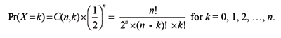
With 10 tosses, it is easy to see that the relative frequencies of heads and tails will only fall within the range of 50 ± 2% if we toss both heads and tails five out of 10 times. The probability of this is the same as the probability of tossing exactly five heads in 10 tosses. Since the number of different ways you can toss exactly k heads in n tosses is given by
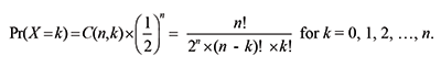
and we are tossing a fair coin, we get the following binomial probability:
For n = 10 and k = 5, this gives us:
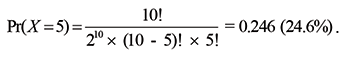
In other words, with 10 tosses, the relative frequencies of heads and tails will still fall outside the interval of 50 ± 2% more than 75% of the time; not really a surprising finding, given that it is perfectly conceivable to throw four heads and six tails in 10 tosses, or vice versa. Clearly, most people who believe that only in the long run will the relative frequencies come close to 50% will expect N to be larger than 10. But how much larger?
People are not likely to expect that the intuitive law of averages applies only to numbers that are far beyond the reach of that very same intuition. What large number of coin tosses would still fall within the “number domain” of their intuition? When I asked members of the choir I sing in for a plausible value of N, most of them suggested that several dozen coin tosses would do. Only one person suggested that it would take as many as 500 coin tosses for the relative frequencies of heads and tails to be reasonably close to 50%, but this number seems more of an educated guess than an intuitive answer.
It appears that most of us intuitively think that the value of N lies in the order of a few dozen coin tosses, but let us not be too strict; say that we intuitively assume that the value of N is approximately equal to 100. Fifty years ago, before the computer age, many textbooks about probability and statistics contained graphs showing that 100 coin tosses are already sufficient for achieving relative frequencies practically equal to 50% (Freudenthal. 1972). Apparently, even mathematically trained people intuitively assume that the value of N is around 100. Is our intuition right? Some math will show.
With 100 tosses, the relative frequencies of heads and tails will fall within the range of 50 ± 2% if X = 48, 49, 50, 51, or 52. Now let Pr(X ≤ k) = Pr(0) + Pr(1) +…+ Pr(k) be the cumulative binomial probability for k = 0, 1, 2, …, n. Then the probability being sought is:
Pr(48 ≤ X ≤ 52) = Pr(X ≤ 52) – Pr(X ≤ 47).
Before the computer age, calculating cumulative binomial probabilities was a laborious task, but today, many statistical calculators on the Internet can do this in no time at all. The probability is 0.691 – 0.308 = 0.383 (38.3%), so—completely contrary to our intuition—at 100 coin tosses, the relative frequencies of heads and tails will still fall outside the chosen interval almost 62% of the time. The mathematician and pedagogue Hans Freudenthal already pointed out this surprising finding some 50 years ago. The best you can say about 100 tosses is that with a probability of 95%, the relative frequencies of heads and tails will fall somewhere between 40% and 60%.
Now, what about 1,000 tosses of a fair coin? This number is much larger than the numbers we are used to dealing with in Bernoulli processes, such as tossing a coin, or betting on the red or black numbers in roulette. Since intuition reverts to what is familiar, it would be exceptional if someone would intuitively conceive of such a large number of tosses or bets. But even if someone did, it would not be of much help. Calculations show that if you flip the coin 1,000 times, there is still a substantial chance of about 20% that the relative frequencies of heads and tails fall would outside the chosen range. To be 95% sure that the relative frequencies fall within the range of 50 ± 2%, you have to toss the coin about 2,500 times! With a smaller interval or a higher probability, the value of N would have been even higher. Would you ever have thought that?
In the Grip of the Gambler’s Fallacy
What does all of this mean? If you intuitively expect the value of N to be somewhere around 100 tosses, which seems a reasonable upper limit for most of us, then the actual difference between the number of heads and the number of tails will be at most 52 – 48 = 4. But with 100 tosses, as seen earlier, it is almost certain that a run of five or more heads or tails in a row will occur and even the probability of a run of seven or more heads or tails in a row is more than 50%. As a result, some kind of compensation for these runs of the same outcome seems to be inevitable. It follows that even the less naïve among us are driven into the arms of the gambler’s fallacy!
Someone might say this kind of reasoning means being doomed to committing the gambler’s fallacy, even if we would intuitively assume N to be very large. After all, the longer we keep tossing a coin, the longer runs of the same outcome are to be expected. There must be some kind of built-in compensation mechanism in Bernoulli processes such as tossing a coin.
This would be true if the length of these runs grew in proportion to the number of tosses, but Schilling shows that the expected length of the longest run of heads or tails in n coin tosses (Rn) is approximately a logarithmic function of the number of tosses: Rn ≈ log2(n). This approximation only gets better with larger numbers of tosses. If we keep tossing a coin, the actual difference between the number of heads and the number of tails will—as a result of these runs of the same outcome—tend to become larger and larger. But because the length of these runs tends to grow only logarithmically, they are increasingly absorbed into the average. As a result, the relative frequencies of heads and tails tend to get closer and closer to 50%. No built-in compensation mechanism is needed.
In short, by bearing in mind that the intuitive law of averages applies to numbers that go far beyond familiar “everyday numbers,” we may escape the grip of the gambler’s fallacy.
Conclusion
Whatever superstitions or cognitive biases about luck dwell in the dark recesses of our minds, the gambler’s fallacy finds its explanation not in the psychology of human judgment, but in the intuitive misapplication of a law of probability. When tossing a fair coin, most of us imagine an irregular but more or less balanced sequence of heads and tails, because we intuitively expect the law of large numbers to manifest itself already in the course of about 100 coin tosses. This is, however, a great misconception.
Mathematics shows that long runs of the same outcome are characteristic of random processes such as the flip of a fair coin. Mathematics also shows that the law of large numbers only manifests itself far beyond the horizon of the numbers we deal with in games of chance or in daily life. Gamblers who pin their hopes on the law of large numbers do so in vain. This surprising discrepancy between the expectations of stochastic intuition and the hard facts of mathematics is a guaranteed recipe for committing the gambler’s fallacy—a fallacy that is difficult to eradicate, not because it is the result of the psychological make-up of human judgment, but because it is rooted in the intuitive understanding of mathematical probability itself.
Further Reading
Bernoulli, J. 2006. The Art of Conjecturing, trans. by Sylla, E.D. Baltimore: Johns Hopkins University Press.
Kahneman, D. 2012. Thinking, Fast and Slow. London/New York: Penguin Books Ltd.
Laplace, P.-S. 1995. Philosophical Essay of Probabilities, trans. by Dale, A.I. New York: Springer Verlag.
Schilling, M. 1990. The Longest Run of Heads. College Mathematics Journal 21(3), 196–207.
Tijms, H. 2021. Basic Probability. What Every Math Student Should Know, Second Edition. New Jersey/London/Singapore: World Scientific.
Tversky, A., and Kahneman, D. 1971. Belief in the Law of Small Numbers. Psychological Bulletin 76 (2), 105–110.
Tversky, A., and Kahneman, D. 1974. Judgment under Uncertainty: Heuristics and Biases. Science 185, 1124–1131.
About the Author
Steven Tijms studied mathematics, classics, and philosophy at Leiden University (The Netherlands). He is especially interested in the border area between mathematics and everyday life, and in the history of mathematics. In classics, his focus is on Latin literature and Neo-Latin texts. He is a tutor of mathematics and the author of Chance, Logic and Intuition. An Introduction to the Counter-intuitive Logic of Chance (2021. Singapore/NewJersey/London: World Scientific).


