
Modeling the Economic and Societal Impact of Non-Pharmaceutical Interventions During the COVID-19 Pandemic

Like many countries affected by the COVID-19 pandemic, the United Kingdom (UK) has deployed a series of national and local Non-Pharmaceutical Interventions (NPIs) in an effort to control the spread of the virus. While others have analyzed the epidemiological impact on, for example, cases and hospitalizations, the broader economic and societal impact can be considered by asking whether, in simple terms, light can be shed on the cost of these measures.
The research goals for this project were:
1.Many important economic indicators, such as the unemployment rate and Gross Domestic Product (GDP), come with a delay of several months. Can statistical modeling be used to infer what these values are today, given historic values up to a few months ago?
2. What impact did an NPI have on a given region? For example, how much did school closures reduce spending? One way to assess such an impact is a randomized control trial: Split the region into two parts, only restrict one part, and measure the difference. Since that isn’t appropriate here, can we use statistical modeling to infer what an unrestricted region would have been like after an intervention date, given historic pre-intervention values?
To answer question 1, nowcasting could be used where models forecast the delayed figures into the present, as illustrated in Figure 1. This provides a delayed target series up to some horizon. The model can be trained to the left of the horizon and use that model to nowcast the target beyond it.
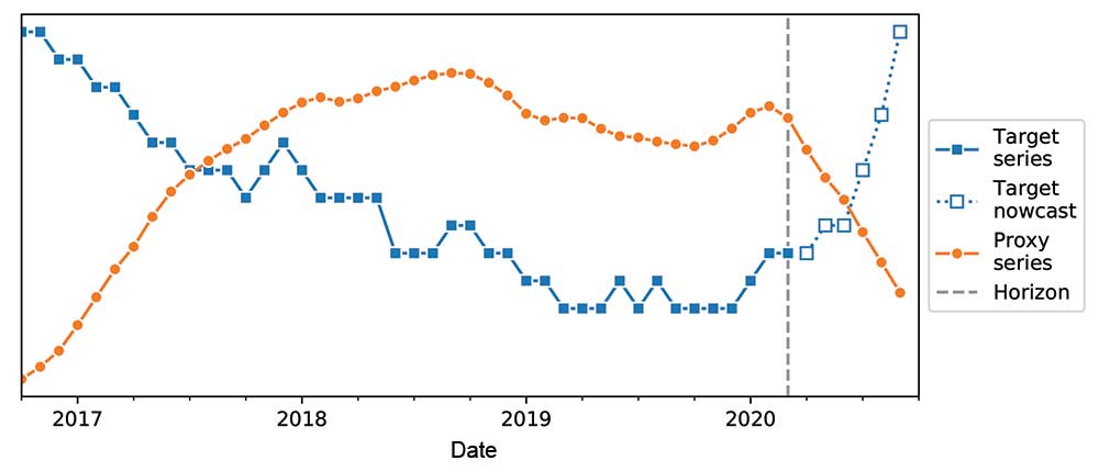
Figure 1. Illustration of nowcasting.
The key difference with regular forecasting is that the horizon is in the past. A related but more up-to-date proxy series (e.g., Google search trends for a topic, rather than the official statistics of that topic) can be taken beyond that horizon up to the present and used in these models.
For the second question, statistical modeling could be used to create a synthetic control. That is, model an alternative, “counterfactual” reality without the NPIs of interest. Predictions can be made about relevant target series, such as the employment rate or spending, in this synthetic region. By measuring the difference between the counterfactual outcomes and the true levels, the impact of the intervention can be inferred.
Notice that building the counterfactual model is essentially nowcasting. Referring to Figure 1 again, the horizon is where the intervention is made, and there is an unrestricted target series up to that horizon. Initially ignoring the target after the horizon, train the model pre-intervention and nowcast past that intervention to create counterfactual values. The nowcast can now be compared to the observed values. If related features are unaffected by the intervention, their post-horizon values can be used in the model just like before.
Before describing the modeling technique used in the nowcasting, it would help to run through some of the data sets to be used in the examples.
Unemployment Rate
A key economic measure is the unemployment rate, which can be determined using data from the International Labour Organization (ILO) and the UK’s Office for National Statistics’ Labour Force Survey. The data are monthly and go back 50 years. There is about a three-month delay, so these data are a prime candidate for nowcasting.
Google Mobility
Modeling societal impact can be illustrated with Google Mobility. The data have been available since early 2020 and show percentage change in visits to places like grocery stores and parks relative to a January 2020 baseline. Being available at the regional level makes the data a good candidates for counterfactual modeling. The impact of an NPI on a region can be understood if, for example, something can be said about the change in the number of visits to shops and supermarkets.
Stock Prices
For the first of the proxy measures (that is, plausibly related measures that have figures up to the present), looking at stock prices and taking the FTSE100—an index on the top 100 companies on the London Stock Exchange—provides a standard indicator of the UK stock market. The FTSE AIM—a similar index but for smaller companies listed on the Alternative Investment Market—can be used to capture the performance of smaller firms.
Google Trends
The next proxy measure is Google Trends, which are trends in Google search terms and can be filtered by country. Google also provides search topics based on groups of related words among languages. Focusing on “unemployment benefits” and “redundancies” topics and working with these trends presents challenges with normalization and uncertainty. Google obfuscates the true number of searches by making only normalized samples of the actual search values available.
A query to Google Trends consists of a date range, geographic location, and search topic. The returned time series are always normalized to have maximum value 100, regardless of the true number of searches. In addition, the returned time series for a given query are a random sample, so the same query does not produce precisely the same time series each time it is made.
The particular concern here is uncertainty in the values, as illustrated in Figure 2. Here, the gray lines are several queries for the same topic over the same period of January 2007 to December 2020. Variation in the values can be seen with each query, so a summary of the distribution of the samples in these models can be used and the (marginal) mean and standard deviation at each time step can be chosen, shown in orange.
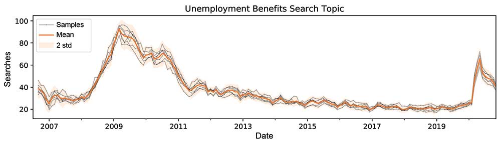
Figure 2. Uncertainty in Google trends results.
Methods
Recall the similarities between the two research goals being considered.
1. The target variables are time series (daily or monthly). The goal is to train models on a period up to a given date and make predictions on a period after that date.
2. There are a number of exogenous regressors, which are also time series, and observations of these variables are available for the training and prediction periods. Predictions for the target variable time series are constructed, in part, from the exogenous regressors.
For both research goals, it would be ideal for predictions to come with confidence intervals (CIs) that capture as much of the uncertainty as possible. The key difference between the two research goals is that in the first goal, the model is designed to predict actual values of the target variable for the recent past and the present; in the second goal, the model is designed to make target value predictions about an unobserved counterfactual world.
While this seems to be a fundamental difference, it actually comes down to the choice of which exogenous regressors to use.
When building any nowcasting model, it is assumed that the same relationship that holds between regressors and the target series during the training period continues to hold in the prediction period. A similar assumption is made with counterfactual modeling, albeit now the assumption is that the relationship would have persisted had the intervention not been made. However, counterfactual modeling makes a further assumption that the exogenous regressors are unaffected by the intervention. In some sense, the regressors likely to satisfy the first assumption are likely to fail here.
To illustrate this, suppose there is a chain of stores in cities across the USA. The San Francisco, California, branch is always late with its profit figures, but the figures from the Los Angeles, California, store, which is always prompt in providing its records, can provide a good idea. This is nowcasting.
Now, suppose there is a promotion in all of the California stores for April. The goal is to know how that affected profits in San Francisco by modeling what the profits would have been without the promotion. LA is a good predictor, but cannot be used here because it has the same promotion. Instead, look at San Francisco sales before April and find another store to use in the model that did not run the promotion.
It turns out the Portland, Oregon, store is also a good predictor, so a similar method can be used by replacing LA with Portland. This is counterfactual modeling.
Nowcasting
The first research goal is to estimate unemployment in December based on the unemployment that can be seen up to September and any other potentially useful values that are available up to the present (i.e., January). This can use the FTSE100 share index, FTSE AIM Index, and Google Trends topics for “unemployment benefits” and “redundancies.”
Figure 3 shows unemployment in the UK over the last 13 years alongside Google Trends data on unemployment benefits. While the searches are not a perfect indicator of actual unemployment, there is clearly a correlation and it should be possible to make good use of the search figures in a model to predict actual unemployment.
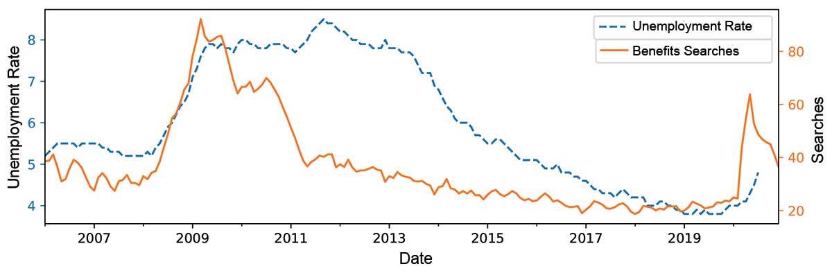
Figure 3. Comparing unemployment and unemployment benefits searches.
Counterfactual Modeling
Bearing in mind the extra assumption on exogenous regressors, to build counterfactual models for a restricted region requires finding other, unrestricted regions that appear similar for the time before the local intervention and use them to train a model for forecasting beyond the intervention.
This can be illustrated with the situation in Leicester over the summer. The blue line in Figure 4 shows the percentage increase in time spent at home relative to a pre-lockdown baseline. As expected, there is a strong weekly seasonality, with the relative increase in time spent at home being much greater for weekdays than weekends, due to a significant decrease in weekday travel for work. After a spike in cases in late June, extra restrictions were placed on the city, as shown by the vertical dashed line.
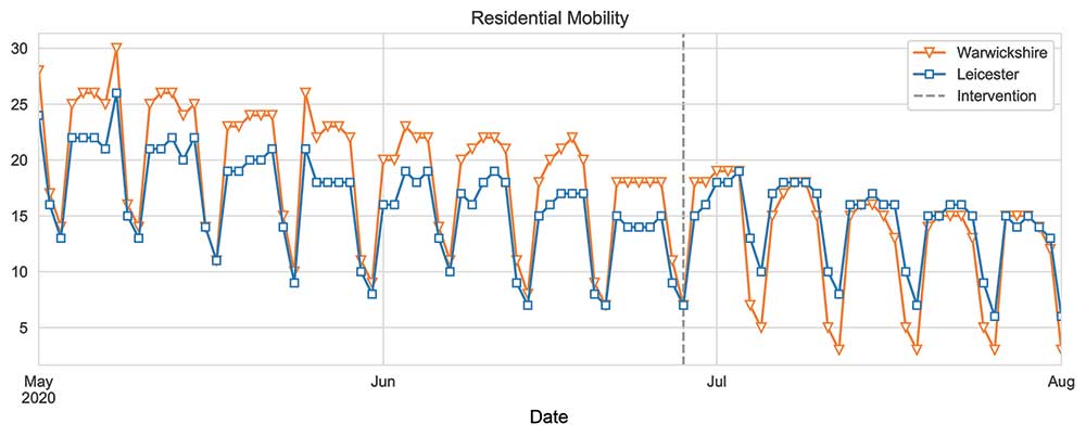
Figure 4. Residential mobility in Leicester and Warwickshire
The aim is to build a model on data before the intervention using regions that look similar to Leicester during the pre-intervention period. Warwickshire, shown in orange, correlates very strongly with Leicester in the pre-intervention period and the restrictions in Warwickshire remained the same throughout the entire period shown in the figure. It can be seen how Warwickshire could be used to “forecast” a counterfactual Leicester beyond the intervention date, supposing that no extra restrictions had been imposed on Leicester.
In general, the few unaffected regions (those without any extra restrictions) whose mobility most closely correlates with mobility in a given affected region (on which restrictions were imposed) can be selected. Warwickshire is one example when Leicester is the affected region.
Gaussian Process Regression
Gaussian process (GP) regression is a Bayesian non-parametric approach to regression with some considerable advantages over other common approaches to regression:
1. Weaker assumptions are made about the relationship between regressors and the target variable. A rich class of non-linear relationships is possible.
2. Uncertainty due to observation noise and extrapolation away from the training data are captured in a principled fashion.
Standard regression is characterized by the following equation:
yi = ⨍ (xi) + ϵi
On observing xis and yis, it can be believed that yis are obtained from xis by first applying an unknown function ⨍ and then adding some (ideally small) corrupting Gaussian noise. Being Bayesian means keeping ⨍ as “unknown” and combining the prior knowledge of how it might look with the observed data to obtain a best posterior “guess.” To do this requires a prior probability distribution over functions that can be crafted to contain the knowledge about f but is not too restrictive.
For example, it might be known that ⨍ is periodic, but it should not be forced to be a sine-wave. GPs are well-suited for this role. Just as a Gaussian distribution is specified completely by its mean and covariance matrix, so a GP is specified by its mean function m and covariance function k.
Suppose ⨍ is believed to be periodic with period 1.
A GP prior could be chosen with the following covariance function:
k(x,x′) = exp(-sin2π|x – x′|) (1)
and m = 0. It is common to refer to the covariance function of a GP prior as a kernel function. The covariance function is maximum whenever the two points x and x′ are separated by an integer distance. The choice of kernel function in equation (1) neatly expresses the prior belief that ⨍ repeats along the x axis with period 1.
Figure 5 shows some random samples from a GP with the covariance function given in equation (1). To form these samples, take some evenly spaced x values x1, x2, …, xn and form the multivariate Gaussian N(μ,Σ), where μi = m(xi) and Σij = k(xi,xj), and then a single sample from this Gaussian gives the corresponding ⨍ (x) values ⨍ (x1),…, ⨍ (xn).
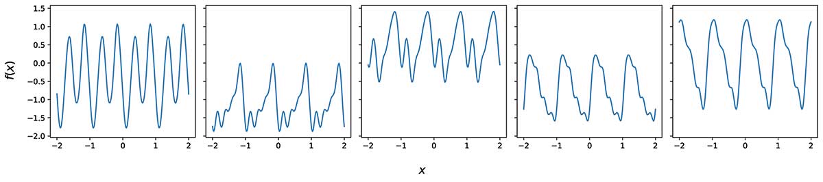
Figure 5. Samples from a simple periodic GP prior.
Note the diversity between samples but the common feature of periodicity with period 1. If the periodicity a priori is not known, it could instead be treated as an unknown hyperparameter and tweaked to get a good fit.
Figure 6 shows a simple example of a GP regression posterior on synthetic sinusoidal data. Note the pleasingly calibrated uncertainty, with the confidence intervals being pinched around the observations, falling back to the prior (mean 0, variance 1) away from the observations and varying continuously in-between. This is a strength of GP regression over other methods: It elegantly quantifies the uncertainty in the predictions, based on how similar the regressors are to previously observed values.
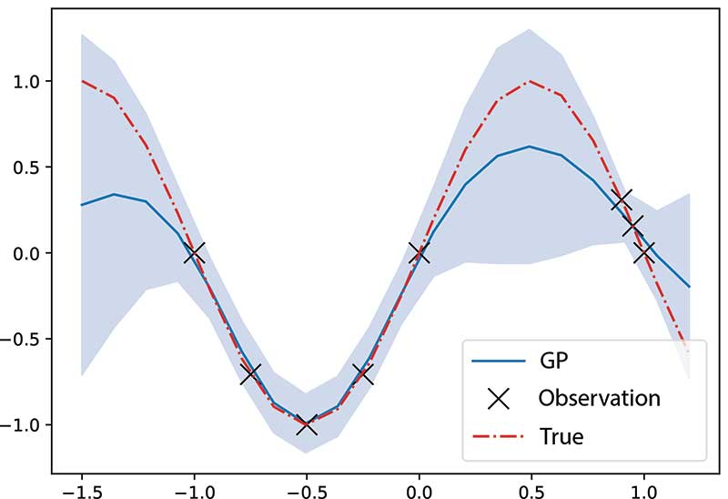
Figure 6. Simple GP regression.
Gaussian Process Regression for Time Series
GP regression can address time series modeling problems such as considered here. There are three approaches:
1. Include time as a variable (e.g., as the number of days since some reference day).
2. Include autoregressive features (i.e., predictions of y can depend on earlier observed or predicted y values).
3. Ignore time and hope that the exogenous regressors can capture the temporal behavior.
After experimenting extensively with each approach, the third approach had the advantage of being the most parsimonious, but one of the other approaches typically yields the best results.
The choice of kernel function for GP regression is key to successful modeling. There are a few defaults for a first attempt at a problem, but more-sophisticated kernels can be constructed by combining simple kernels in products and sums. Separable kernels can be found to be successful for these problems.
In the first approach, the regressors are the exogenous regressors x (Google Trends, FTSE, other regions’ mobilities) and a time variable t, denoting the day or month. A good kernel structure is one where the overall kernel can be written as a product of the kernel on each variable type:
k((x,t),(x′,t′)) = kX (x,x′) kT (t,t′) (2)
where kT has components including periodic kernels and linear trends, and kX is some general-purpose kernel. This structure reflects our assumption that the relationship between exogenous regressors and the target does not vary over time. A related structure in the case of approach two is:
k((x,y),(x′,y′)) = kX (x,x′) kY (y,y′) (3)
where x and y refer to the exogenous and autoregressive features, and each kernel is a general-purpose choice. Equation (3) reflects a more-subtle assumption: The target variable can depend on earlier values of itself (autoregression) and on exogenous regressors, but there is no interaction between the two. This can continue in this manner and encode yet more structure, such as:
k((x,y,t),(x′,y′,t′)) = kX (x,x′) kY (y,y′) + kT (t, t′) (4)
where a periodic time kernel augments the previous kernel structure with some additive seasonality.
Figure 7 shows some random samples from a time-dependent GP prior that can be used in practice. These plots are not supposed to look like any specific unemployment time series, but they demonstrate some of the variety of time series that the priors encode (multi-scale periodicity, global trends, dramatic spikes, etc.).
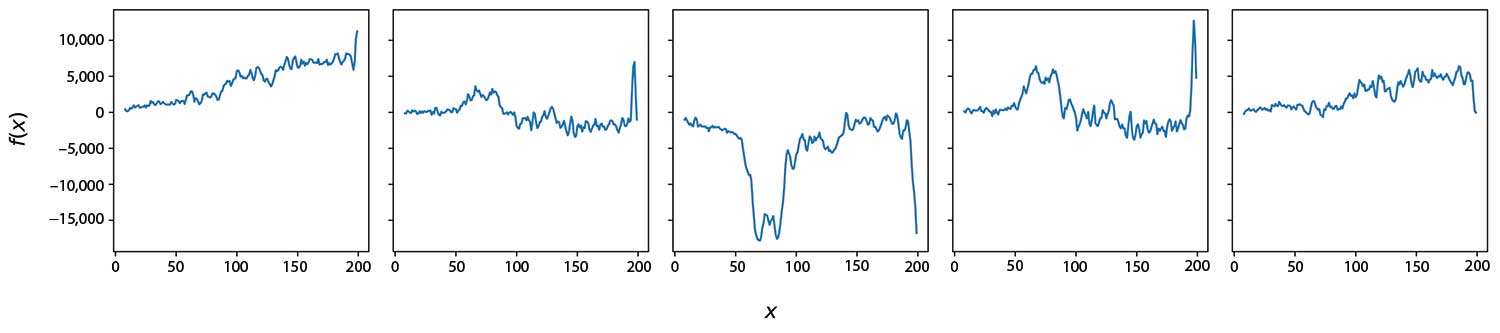
Figure 7. Samples from a GP prior used in the models.
Input Uncertainty for Gaussian Process Regression
In a standard regression set-up, the regressors (or inputs) are known exactly. Consider using FTSE100 values as a regressor for unemployment; the high, low, open, and close prices of the FTSE100 are known exactly for each day. By contrast, the Google Trends data are inherently and unavoidably uncertain, possessing a mean and variance for each time step. For the UK, the uncertainty in important search terms is not negligible and varies over time. Neglecting it and using only the mean could underestimate the predictive uncertainty, but also lead to models that fixate on spurious minor variations in the mean.
Standard GP regression does not naturally accommodate uncertainty on the regressors, but a few techniques have been studied. One such technique, introduced by McHutchon and Rasmussen (2011), is the noisy input GP (NIGP), which assumes the regressor uncertainty to be Gaussian and relatively small in magnitude, meaning that a Taylor expansion can be used on the unknown regression function
![]()
Although elegant, this technique is rather limited, requiring the regressor uncertainty to be the same at each point and being limited to a few special and simple kernel functions for which the distribution of the derivative in (5) can be computed by manual calculus. A generalized version of this method, the heteroskedastic NIGP (HNIGP), can have variable uncertainty across data points and any choice of kernel function.
Briefly, heteroskedasticity is obtained by promoting ε to a function of x and extending to general kernel functions by using automatic differentiation in a modern deep learning framework to compute the derivative in (5). (The HNIGP will be described in full in a forthcoming technical report.)
Other Models
Some alternative modeling approaches complemented and strengthened the analysis using GP models. For unemployment nowcasting, a very classical approach is an autoregressive integrated moving average model (ARIMA) and in particular SARIMAX: seasonal ARIMA with exogenous regressors. These models are simple by comparison with GPs, being parametric and linear, but can nevertheless be quite effective (Brockwell and Davis. 1991). In the case of counterfactual modeling, refer to a method from Broderson, et al. (2015) in “Inferring causal impact using Bayesian structural time-series models.” Their method, called Causal Impact, is a Bayesian structural time series approach with linear regression on exogenous regressors.
The final approach—synthetic control—is frequentist and linear, and was developed over a series of papers by Alberto Abadie and collaborators (2011. Journal of Statistical Software, accompanying the R package Synth). SARIMAX and causal impact predictions come with uncertainty estimates, but these do not account for as many sources of uncertainty as GP regression.
Evaluation
Whether the models make correct predictions and reliable uncertainty estimates must be verified. Using GP regression provides some assurance of a model’s behavior and how uncertainties will be handled, but it is still possible to construct models that make bad predictions. Such evaluation needs a ground-truth and a means of scoring the predictions against that ground truth.
First, look at scoring metrics. To compare predictions to the truth, the familiar root-mean-squared-error (RMSE) can be used, which measures the difference between the predictions and observations intuitively. However, it should be emphasized that while producing inaccurate predictions is bad, being confident in those bad predictions is worse. The models should be able to shrug and say, “I don’t know” by producing predictions with wide confidence intervals.
RMSE neglects uncertainty, so negative log-likelihood (NLL) is also considered, which measures how likely the observations are given the mean and variance of the predictions. Figure 8 gives an illustration of RMSE and NLL, showing example predictions that give high and low scores for each scoring metric. With a selection of model types, GP kernels, regressor choices, and data pre-processing, the best model can be selected by performance on some appropriately chosen test data.
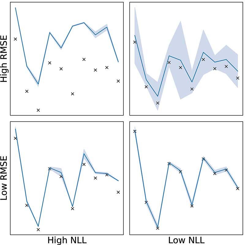
Figure 8. Illustration of RMSE and NLL scores in backtesting.
If the chosen best model’s predictive confidence intervals reliably contain the targets in the test data, there can be confidence that the same model, when used to make genuine nowcasts or counterfactual predictions, will produce trustworthy predictions and confidence intervals.
In general, NLL would be used when validating modeling choices—like kernel design—and RMSE when reporting results in an understandable way.
Having established some scoring metrics and methodology, it is time to find some test data. In many standard machine learning problems, models are verified on a held-out test set of data that the model has not seen during training. Neither of these problems presents an obvious way to split the data into training and test. Nowcasting would have to be evaluated on as-yet unobserved values. Counterfactual modeling would require being evaluated on a fictitious UK from a parallel universe!
Nowcasts
The process of backtesting can be adopted to evaluate the nowcast models, an approach often used in financial modeling. Say there are unemployment data for up to November 2020. To nowcast up to the present (January, at the time of writing) requires using the models to predict two time-steps ahead (December, January).
Fixing everything else about a model, we could instead train up to September, leaving October and November unused. The model’s predictions could then be compared for those two months against the observations using RMSE and NLL. This process could by repeated by going further back a few more time-steps, thereby producing several sets of predictions and scores. The best model attained RMSEs over five backtests varying between 0.05 and 0.15 percent, at unemployment values of between 4 and 5 percent.
Counterfactuals
Obtaining appropriate test data for the counterfactual models seems impossible at first glance since, by definition, their predictions pertain to an imaginary UK in which the COVID-19 restrictions were different from those actually imposed in the real UK. Instead, take the same approach as above and predict things that can be observed, changing the problem into a regular nowcast one.
- Change time: Conduct a test using a placebo intervention date one month before the actual intervention date. The predictions can be compared against the observed values for the next 30 days.
- Change space: Conduct a placebo test that treats a region without restrictions as if it were restricted. As before, model the area using other areas without restrictions and compare the predictions with the observed values.
Figures 9 and 10 illustrate these two approaches. In these plots, the top panel shows observed percentage change in mobility as a solid, black line and the model’s predictions as a dashed, blue line that is shaded 95 percent CI. The intervention dates are shown as a dashed, vertical, black line; the models are trained on data to the left of this line. The bottom panel in these plots shows the difference between observations and predictions, which is the “effect” of the intervention.
Figure 9 imagines that restrictions in Leicester came a month early. Notice how the prediction continues to track reality up to the true intervention date. Figure 10 applies the same modeling to Nottingham, which was unrestricted throughout this period. Again, predictions match the truth.
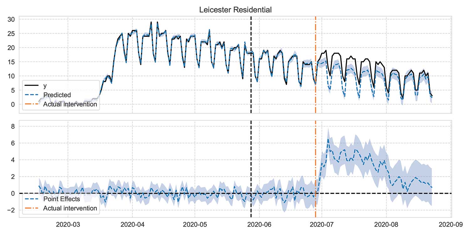
Figure 9. Validating counterfactual prediction by moving the intervention date, illustrated by percentage change in residential mobility. Vertical, dot-dashed, orange line shows = true date = when new restrictions were imposed; black dashed vertical line shows chosen placebo intervention date.
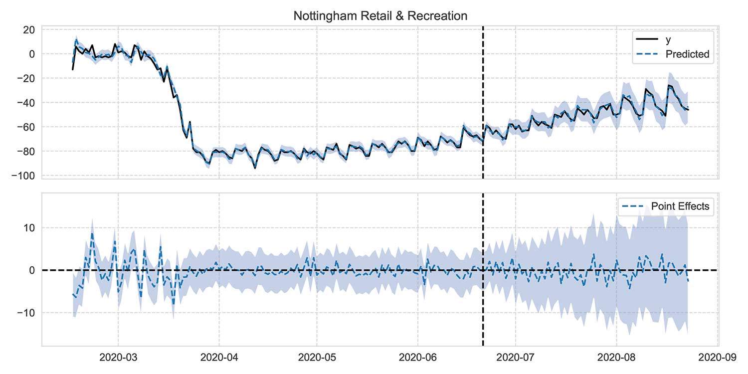
Figure 10. Counterfactual prediction on regions without interventions, illustrated by percentage change in retail and recreation mobility. Black dashed vertical line shows chosen placebo intervention date.
Since the UK has more than 300 regions, it does not require backtesting to boost the test data; simply perform similar validation across all regions and look at the distribution of values. As suggested by these examples, the model has good performance on Google Mobility data. We estimate the predictions to be accurate to within one or two percentage points.
These results provide confidence in the counterfactual predictions, in particular by ruling out any tendency of the models to systematically over- or under-predict. What is more, the accuracy of the predictions on regions that did not see any extra restrictions validates the assumption that these regions are unaffected by the extra restrictions introduced in other regions.
Results—Unemployment Nowcasts
The best model for nowcasting unemployment is based on the backtests. Results are in Figure 11, showing the RMSE and NLL summarized over all of the stepped backtests by mean and standard deviation.
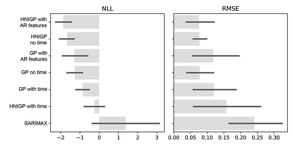
Figure 11. Backtest results for unemployment nowcasts plotting the mean and two standard deviations over five stepped backtests for each model variant.
The winning model was a GP with input uncertainty and some autoregression (“HNIGP with AR features” in the plot). This model has the lowest NLL and RMSE; we are biased toward models that account for input uncertainty unless there is convincing evidence to reject them.
Explicitly, the kernel was the one in equation (4), with both kX and kY being the sum of a standard radial basis function (RBF) kernel with automatic relevance determination (ARD) and a linear kernel. Over several stepped backtests, the model’s predictive confidence intervals always contained the true observed values. The true value of unemployment at the end of November 2020 was 5.0 percent and, using Google Trends and stock market data available at the end of January 2021, the model predicted an increase to 5.2 percent by the end of January (95 percent CI 5.0 to 5.4 percent).
Figure 12 shows the predictions of the model over the past few years (blue line) and up to January 2021 against the observed values (black dots).
Results for models without any exogenous regressors, just treating the time series as an isolated process, are noticeably worse, showing that the external information from Google Trends and the stock market are adding value to the model. Similarly, ignoring input uncertainty results in worse fits and, counterintuitively, larger confidence intervals in December and January. This is a clear sign that accounting for input uncertainty protects models against fixating on insignificant small variations in the training data.
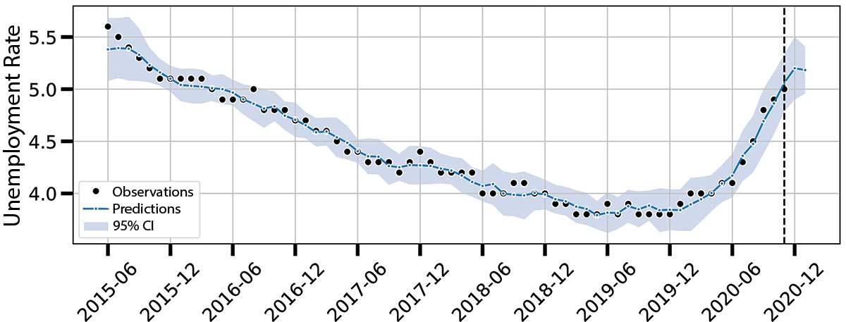
Figure 12. Unemployment rate model predictions.
Local Restrictions
As a result of the counterfactual modeling and validation described above, we can make confident predictions of the impact of NPIs in various regions. Rather than provide all UK regions or types of mobility here, these are some illustrative examples.
Sticking with the Leicester example, Figure 13 shows residential mobility (relative increase in time spent at home) before and after the introduction of the extra restrictions (black vertical line). In the week after the summer restrictions, time spent at home (solid black line) was 5 percentage points (95 percent CI 4 pp to 6 pp) higher than it would have been had the extra restrictions not been imposed (dashed blue line and shaded 95 percent CI region).
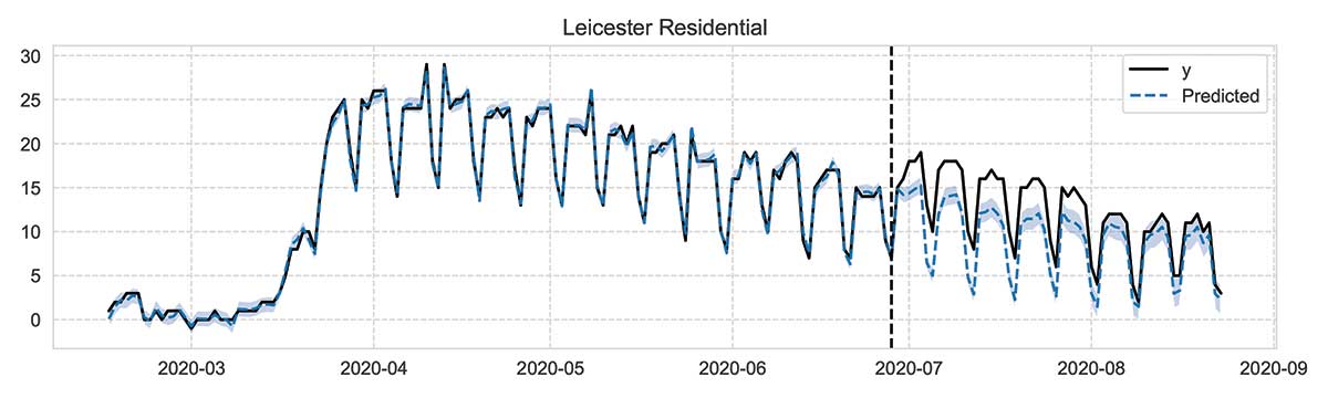
Figure 13. Plot of relative change in residential mobility (time spent at home) in Leicester over six-month period. Vertical dashed line indicates introduction of stronger restrictions in the city. Plot contrasts observed mobility with counterfactual predictions supposing restrictions had not been imposed.
To reemphasize, the blue dashed line shows the counterfactual predictions after the intervention date, and the solid black line shows the actual observed mobility in the same period. The same analysis for retail and recreation locations shows that visits were down by 20 pp (95 percent CI 15 pp to 25 pp) as a result of the summer interventions. Local restrictions such as those considered here are a devolved issue; in England and Scotland, regional NPIs are implemented as tiers, with regions in a given tier given a common set of NPIs.
The models can be used to make statements about, say, the impact of Tier 3 over Tier 2 in England, by building a counterfactual model for each Tier 3 region, supposing that it had remained in Tier 2, and aggregating the results into a single estimate. Doing so finds that in the week after the introduction of tiers in October 2020, visits to workplaces in a Tier 3 region were 10 pp (95 percent CI 6 pp to 14 pp) lower than if the same region had remained in Tier 2. On the other hand, there was no significant impact on visits to parks.
Conclusions
These examples illustrate the similarities between nowcasting and counterfactual modeling; a difference that rests solely in the choice of exogenous regressors. It is clear that counterfactual modeling can infer the impact of NPIs in the UK in recent months and how key indicators of economic health can be tracked in real time without waiting for official figures to be released.
Gaussian process regression handles implementing uncertainty in various aspects of modeling in a natural and principled way. The validation is important, and sometimes creativity is needed to find validation data, particularly with counterfactual modeling.
Finally, these nowcast and counterfactual models can be applied to other data. Thanks to robust validation and handling of uncertainty, the performance on any new data can be judged to provide and give confidence in any predictions—even if the data cannot be modeled, the validation and confidence intervals should reflect this.
Further Reading
Brockwell, Peter, and Davis, Richard. 1991. Time series: theory and methods. New York: Springer-Verlag.
Brodersen, Kay H., et al. 2015. Inferring causal impact using Bayesian structural time-series models. Annals of Applied Statistics.
McHutchon, Andrew, and Rasmussen, Carl. 2011. Gaussian process training with input noise. Advances in Neural Information Processing Systems.
Williams, Christopher, and Rasmussen, Carl. 2006. Gaussian processes for machine learning. Cambridge, MA: MIT Press.
About the Authors
Jon T. is technical director of the Artificial Intelligence Lab at Government Communication Headquarters (GCHQ). Previously, he led the Machine Learning team in GCHQ’s Research, Innovation, and Futures division. His research interests focus on Bayesian machine learning and its practical application to operational problems.
Nicholas B. is a machine learning researcher and data scientist in the Research, Innovation, and Futures division of GCHQ. His research has focused on machine learning for speech and natural language processing, data triage, Bayesian machine learning, and deep learning theory. He has also worked extensively on practical data science projects.
Thomas Middleton is a data scientist in the Cabinet Office, a UK government department based in London and tasked with supporting the prime minister and ensuring the effective running of government. He has a PhD in economics from the University of Kent and an ongoing research interest in the application of statistical and econometric techniques for policy evaluation.
Editor’s Note: Employees of GCHQ are required to be identified by initial rather than last name.


