
Statistical Analysis of the Elo Rating System in Chess

The World Chess Federation (FIDE) and many other chess organizations use the Elo rating system to quantify the relative ability of chess players. The system was originally devised by Arpand Elo (1903–92) and is detailed in his book The Rating of Chessplayers, Past and Present (Elo. 1978). FIDE adopted the Elo rating system in 1970 and has used it ever since, but, more recently, more-sophisticated and seemingly superior rating systems have emerged, such as the proprietary TrueSkill rating system developed by Microsoft Research (Herbrich, et al. 2007), the Glicko rating system developed by Harvard statistician Mark Glickman (Glickman, n.d.), and the Chessmetrics rating system constructed by Jeff Sonas. Nonetheless, the Elo system remains the standard rating system used in chess, and its properties are of interest to statisticians.
A little over a year ago, on February 15, 2019, YouTuber and freelance mathematician James Grimes posted a video titled “The Elo Rating System for Chess and Beyond” on his channel singingbanana and it has since garnered more than 270,000 views (Grimes. 2019). This popular video provides a broad overview of the mathematical and statistical characteristics of the Elo rating system and can also serve as a good introduction to this article.
This article details a mathematical and statistical framework for the Elo rating system, filling in some mathematical details left out of the YouTube video, and then analyzes the accuracy of the Elo rating system with real-world data using two chess databases: one containing chess games played by humans and another containing chess games played by computers.
Statistical Framework for the Elo Rating System
In the Elo rating system, if Player A has an Elo rating that is 400 points greater than opponent Player B, then Player A should be 10 times more likely to win the game. More generally, if Player A has rating RA and Player B has rating RB, then the odds of Player A beating Player B are given by the following formula.
![]()
Solving for Pr(A beats B) gives:
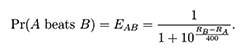 (1)
(1)
This probability can also be interpreted as an expected score for Player A when playing against Player B, shown as EAB above. The three possible outcomes for A are win, lose, or draw, corresponding to scores of 1, 0, and 0.5, respectively.
This article studies the accuracy of the probability statement in Equation (1) by analyzing the prediction errors—the difference between the actual scores and the predicted scores based on Equation (1). More specifically, the prediction error for Player A against Player B is:
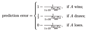 (2)
(2)
One important fact is well-known to most chess players but not reflected in Equation (1): The player who plays with the white pieces, which by the rules of the game means the player who moves first, has a distinct advantage over the player with the black pieces. The quantitative nature of this advantage is analyzed with large chess databases later on in this article, but first, we study the implications of Equation (1) by considering a special statistical model that is governed by the same probability structure provided by Equation (1). More specifically, we shall assume the ratings for players A and B follow independent probability distributions engineered in such a way that a formula similar to Equation (1) arises. The starting point is the Gumbel distribution.
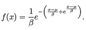
The Gumbel distribution (also known as the type-1 generalized extreme value distribution) with location parameter μ and scale parameter β has the probability density function of:
Furthermore, if A ∼ Gumbel(μA, β) and independently β ∼ Gumbel(μB, β) (with matching scale parameters), then B − A follows a logistic distribution with location parameter μB − μA and scale parameter β. Therefore, the probability Pr(A > B) can be computed with the cumulative distribution function of the logistic random variable B − A, which is given by:
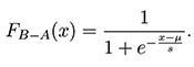 (3)
(3)
Noting the similarity between (3) and (1), a careful choice of μA, μB, and β will allow these expressions to match up. In particular, taking μA = RA, μB = RB, and
![]()
gives
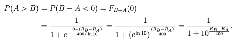
Figure 1 provides a graph of two Gumbel distributions. The modes of these two distributions are 2,000 and 2,500, respectively, and both have the scale parameter 400/ ln(10) ≈ 174. To provide more perspective, the 95% highest density intervals for each distribution is shaded. For example, under this model, a 2,500-rated player would perform in the range [2,229, 3,049] approximately 95% of the time.
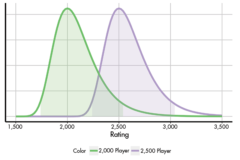
Figure 1. Gumbel distributions with location parameters 2000 and 2500, respectively, and scale parameter 400/ ln 10. The 95% highest density intervals are highlighted.
It is natural to find this statistical model to be rather restrictive—all players have the same distributional form and scale, with the only difference being the location parameter. For example, one might think that players with relatively high ratings might have less variation in performance compared to lower-rated players, suggesting a distributional form that varies with the player’s rating. In addition, modeling the probability of only two outcomes—a win or a loss—is also quite restrictive; chess games against similarly matched opponents will often end in a draw.
Yet, even with these limitations, this rather simplistic and restrictive model produces fairly reasonable approximations.
To round out the discussion of Elo rating, we briefly describe how Elo ratings are updated once a game is finished and an outcome is determined. Suppose Player A with rating RA plays against Player B with rating RB, then the new rating of Player A, denoted R‘A, is given by this formula:
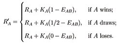
In this formula, EAB is calculated from Equation (1), and KA is some positive constant—referred to as the K-factor—that represents the maximum possible rating adjustment. Therefore, if two players are equally rated and the result is a draw, then the ratings of both players will remain unchanged. However, should Player A win a rated game against Player B, and the two players were equally rated, then Player A would gain KA / 2 rating points and Player B would lose KB / 2 rating points.
Often, the K-factor of the two players will be the same, so the number of rating points gained by one player will equal the number of rating points lost by the other player. However, the K-factor may vary based on the player’s rating (a smaller K-factor is often used for higher-rated players), the number of rated chess games the player has played (a larger K-factor is often used with players who haven’t played many rated games), and time control used (the K-factor may be reduced for higher-rated players in events with shorter time controls).
If the K-factor is set too large, the rating will be overly sensitive to just a few recent events, and if the K-value is too low, the ratings will not respond quickly enough to changes a player’s actual level of performance. FIDE uses a K-factor of 40 for new players to the rating system and a K-factor of 10 for seasoned top-ranked chess players with ratings over 2,400.
Analysis of Results with Highly Rated Chess Players
To evaluate the performance of Equation (1), we analyzed a large database of chess games among chess players with Elo ratings of at least 2,000—in the freely available KingBase database, which contains approximately 2.1 million games played after 1990, collected from various chess tournaments around the world.
Using this database, the prediction error for the player with the white pieces is calculated for every game using Equation (2). The overall average prediction error is 0.0407 with a standard error of 0.000238, suggesting a statistically significant bias for the white player. This bias can be considered comparable to 35 Elo rating points; when 35 points are added to every player with the white pieces in the database, the average prediction error reduces to zero.
The prediction error also may change according to a player’s rating and the difference in ratings between the two players. These effects are studied using a linear regression model. The discreteness of the possible outcomes (win, lose, or draw) produces a bimodal distribution of prediction errors, as depicted in Figure 2.
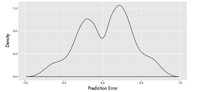
Figure 2. Density of the prediction errors in the KingBase database.
Although normality and other assumptions may not hold exactly when fitting a linear regression model, the model can still yield useful inferences due to the large amount of data available. A linear regression model can be used to assess the effect of the white player’s Elo rating and the difference between the white and black players’ Elo ratings on the prediction errors. These two regression variables are mean and standard deviation-normalized to allow for better interpretation of the regression coefficients.
The fitted regression equation is:
![]() (4)
(4)
The 95% confidence intervals for the estimated regression coefficients are (0.0402, 0.0411) for the intercept term, (0.00605, 0.00712) for white player’s standardized Elo rating, and (-0.0175, -0.0164) for the standardized Elo rating gap. Although all three regression coefficients are highly statistically significant due to the extremely large sample size of the database, the effects of the two regressors are not particularly large when compared to the intercept term. More specifically, the advantage of going first, represented by the intercept term, dominates the other effects.
The positive regression coefficient 0.00658 suggests that Equation (1) slightly under-predicts the expected score for players rated above the database average rating of 2,358. Similarly, the negative regression coefficient of -0.0170 suggests that Equation (1) slightly over-predicts the expected score when facing an opponent with a lower rating. With a large rating gap, this effect can be fairly substantial. For example, the advantage of going first as a player with the white pieces is negated when playing against an opponent with an Elo rating that is 417 points lower.
Figure 3 shows the density of the modeled prediction errors across the entire database. The distribution is centered around 0.0407, which represents the advantage of going first, and ranges from 0 to 0.08. Although mismatched ratings can introduce bias in the prediction errors, this bias is relatively small in comparison with the overall average.
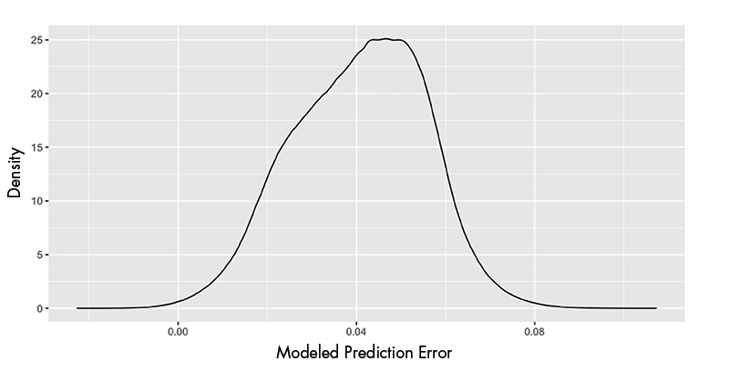
Figure 3. Density of the modeled prediction errors for the player with the white pieces based on Equation (3).
Suppose a chess player with a 2,400 Elo rating plays with the white pieces against the reigning world champion, Magnus Carlsen, who currently holds the world’s highest rating of 2,872 (at the time of writing this article). The prediction error model estimates the prediction error to be 0.0900, which is equivalent to a 2,400-level player actually playing at an Elo rating of 2,573. Carlsen is still very much expected to win the game, but, should he lose, his rating would be overly reduced by 0.897 points, which to him may be considered quite substantial, because he is currently hovering around his peak rating of 2,882 that he obtained many years ago—in May of 2014.
Of course, Carlsen’s rating is at the extreme end of ratings in the database, and the estimated effects may not be as accurate for players of his caliber. There is justification that very highly rated players would put themselves at a disadvantage by playing in open tournaments in which they might be paired against players with substantially lower ratings. Indeed, the very top-ranked chess players are seldom found playing in open tournaments in which they could face significantly lower-rated opponents.
Players also will often carefully prepare for their upcoming games by formulating strategies based on frequently played openings of their opponents, and such personalized preparations can have a dramatic influence on the result of the game. Hence, another practical reason why top-ranked players might avoid open tournaments would be that less preparation is required for opponents one has faced many times previously.
Accounting for Draws
Equation (1) has been shown to be largely accurate, although incorporating the advantage in having the white pieces could significantly improve the rating system. However, predicting the expected score with Equation (1) is not equivalent to predicting the probability of winning the game, since equally rated players often draw their games. The proportion of draws for two players with ratings in the range of 2,000 to 2,900 can now be analyzed.
Figure 4a depicts the proportion of draws for each combination of players within a specified 50-point range, provided at least 50 games were recorded in the database with such a pairing. If fewer than 50 games were played, the respective square was left blank. For equally rated players, the probability of a draw ranges from 35% to 55%, and the proportion of draws increases as the ratings increase.
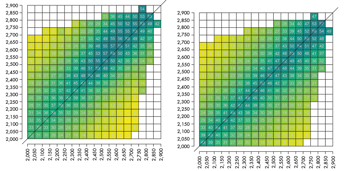
Figure 4a (left). Probability of a draw between two players with ratings ranging from 2,000 to 2,900.
Figure 4b (right). Modeled probability of a draw per Eqn (5).
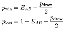
Letting pdraw be the probability of a draw and EAB be the expected score, the probability of a win and loss, denoted by pwin and ploss, respectively, can easily be calculated:
Therefore, a simple model of the probability of draws would be helpful in modeling the probability of a win and loss, not just the expected score. The result of a logistic regression fit that models the probability of a draw based on the Elo rating of the player with the white pieces and the difference in ratings between the two players is:
Pr(draw) = logit−1 (−1.627 + 0.0006955 * Rwhite − 0.004668 * |Rwhite − Rblack|) (5)
where:
![]()
Using this logistic regression model, the probabilities of a draw can be calculated for the entire data set. Figure 4b displays the model-based draw probabilities, and allows for a direct comparison to the observed draw probabilities graphed in Figure 4a. In particular, it can be seen that the logistic regression model reasonably approximates the observed draw probabilities, and that Equation (5) can serve as a reasonable approximation to modeling the probabilities of a draw with two players in the 2,000 to 2,800 Elo range.
Analysis of Computer Chess Games
At this point, for most high-level tournament-going players, there is a fairly substantial advantage for the player with the white pieces that is tantamount to approximately 35 Elo rating points. An “underdog advantage” has been identified in which players with substantially lower Elo ratings compared to their opponents tend to perform better than what is predicted by Equation (1).
Modeling the probability of a draw also finds that equally rated players with Elo ratings of 2,500 and above tend to draw around 50% of their games.
Next is to see how each of these properties may or may not be reflected in a separate database of computer games with engines having “super-human” Elo ratings—ranging from 2,901 to as high as 3,496.
The Computer Chess Rating Lists (CCRLs) website provide more than 1 million chess games played between various computer software programs, with a 40/15 (40 moves in 15 minutes) time control. Limiting this analysis to games played between computer engines with super-human Elo ratings above 2,900 leaves nearly 100,000 games to analyze involving 88 different programs and more than 700 versions of these programs.
With the computer chess database, the average prediction error for white is 0.0513, which equates to approximately a 39 Elo rating point advantage. This is a little higher than the 35 point advantage identified in the previous database. The distribution of the prediction errors for the computer chess games also mimics that of the previous database (data not shown). Interestingly, however, the effect associated with the difference in rating between two engines displays an opposite effect.
More precisely, if the engine with the white pieces has a substantially larger rating compared to its opponent, the probability of a win is higher than what would otherwise be predicted from the probability formula. The fitted regression equation uses the computer chess database and is comparable to Equation (4).
![]() (6)
(6)
As before, since the size of the database is quite large, the estimated coefficients, albeit somewhat small, are all statistically significant; the 95% confidence intervals for the estimated regression coefficients are (0.0494, 0.0532) for the intercept term, (0.000833, 0.00502) for white player’s standardized Elo rating, and (0.0210, 0.0252) for the standardized Elo rating gap.
As an example, the model of the prediction error above suggests that a 3,400 Elo-rated engine with the white pieces that plays against a 3,200-rated engine has the equivalent of a 119 Elo-rating point advantage. It is interesting how the underdog advantage when two humans play each other turns into an underdog disadvantage when two engines play each other.
Finally, the frequency of draws when highly rated computer engines compete against other highly rated engines can be studied. Figure 5 is analogous to Figure 4a and depicts the proportion of draws by computer programs that are within a specified 50-point range—provided at least 50 games were recorded in the database with such a pairing. If fewer than 50 games were played, the respective square was left blank. In particular, the probability of a draw for equally rated engines ranges from 46% all the way up to 84%, with the proportion of draws increasing as the rating increases.

Figure 5. Probability of a draw between two computer engines with ratings ranging from 2,900 to 3,500.
Acknowledgments
The author appreciates the careful and detailed anonymous reviewer comments that led to a much-improved manuscript. The author also appreciates the efforts of Angelina Berg, who provided editorial support.
Further Reading
Elo, A.E. 1978. The Rating of Chessplayers, Past and Present. Arco Pub.
Glickman, M. n.d. The Glicko System.
Grimes, J. 2019. The Elo Rating System for Chess and Beyond.
Herbrich, R., Minka, T., and Graepel, T. 2007. TrueskillTM: A Bayesian Skill Rating System. Advances in Neural Information Processing Systems, 569–576.
About the Author
Arthur Berg is an associate professor in the Division of Biostatistics & Bioinformatics at the Penn State College of Medicine. He is also director of the biostatistics PhD program and an avid chess player (although not a very good one). He regularly teaches a graduate-level Bayesian statistics course, and Bayesian statistics has been his main research interest for the past several years. He also collaborates with many clinician scientists and holds joint appointments in the Departments of Statistics, Family & Community Medicine, Surgery, and Neurosurgery.
Thanks for this great article – I came across it because I was interested in where computer chess may be heading – your last chart is of particular interest.
Do you think computer engines are empirically proving that chess, if played perfectly, always results in a draw?
Could you maybe add a chart of % draws vs ELO?