
Using Differential Comparisons in Observational Studies
 In a randomized experiment (e.g., a randomized clinical trial), a fair coin is flipped to decide whether the next person will be assigned to treatment or control. Because the coin is fair, the chance that any one person will end up in the treated group is the same as the chance of ending up in the control group. Therefore, aside from chance, no type of person is over-represented in the treated or control group. If the difference in outcomes after treatment is too large to be due to chance—too large to be attributed plausibly to an unlucky sequence of coin flips—then a treatment effect
is demonstrated.
Without random assignment, treated and control groups may differ prior to treatment. The groups may differ in ways we can see, they may differ in terms of measured covariates, but it would be naive to suppose they differ only in ways we can see. When treatment effects are estimated from nonrandomized studies, observational studies, most of the controversy concerns possibility that the groups differed prior to treatment in ways we cannot see in measured covariates.
We address biases visible in measured covariates by comparing people who look similar in terms of measured covariates, for instance, by matching treated subjects to controls so treated and control groups looked comparable prior to treatment in terms of measured covariates. People who look comparable in measured covariates may not be comparable, so to address unmeasured biases we need to do more.
What are Differential Comparisons, and What Types of Unmeasured Biases Do They Address?
Where matching removes visible differences in measured covariates by comparing people who are similar, differential comparisons compare people who are visibly different in the hope they are similar in terms of unmeasured covariates. In a sense, differential comparisons overcompensate for observable quantities in an effort to compensate adequately for unmeasured biases. Differential comparisons are easy to do, are quite intuitive, are supported in a specific way for a specific purpose by statistical theory, and are-at worst-a harmless and transparent supplement to standard comparisons of people who look similar. Yet, differential comparisons are rarely done.
My purpose is to illustrate the use of a differential comparison in an example, sketch the underlying statistical idea, and illustrate certain other techniques for observational studies.
The key idea is that certain unmeasured biases, called generic biases, promote more than one treatment in a similar way. If you were studying one such treatment and I were studying another, the generic bias might lead both of us to the wrong answer for the same reason. If we worked together and looked at both treatments at once, perhaps we could see a little more.
With two treatments, each at two levels, treated or control, there are 2 x 2 = 4 combinations of treatments. The differential comparison compares two of the four combinations. The differential comparison sets aside, for a moment, for one analysis, the people who received both treatments and the people who received neither treatment. It then compares the people who received one treatment in lieu of the other.
Under simple models for treatment assignment, the differential effect is less biased than other comparisons by generic biases that promote both treatments. Indeed, the differential effect can be entirely unbiased when a study of either treatment in isolation would be severely biased by the generic bias. Obviously, the differential effect is a comparison of two potentially active treatments, so it is not the effect of either treatment taken in isolation, but with that fact firmly in mind, perhaps we can learn something from the differential comparison.
Some people are careful about what they eat, about the health benefits or harms that may accrue to a poor diet, and others eat what they like. People who are careful about what they eat will often eat less saturated fat and more fiber, less red meat and more vegetables, less fried food and more salad. Before you attribute some health benefit to reduced saturated fat and I attribute it to increased fiber, perhaps we should compare notes, make the differential comparison of a first diet good in terms of saturated fat and bad in terms of fiber with a second diet bad in terms of saturated fat and good in terms of fiber. That comparison will exclude the people most and least dedicated to a healthy diet.
Pointedly, we would be comparing people whose behavior is twice different, differing in both saturated fat and fiber, in the hope that they are similar, similar in terms of moderate dedication to a healthy diet.
In the next section, daily smokers and nonsmokers are compared in terms of toxins found in their blood, the comparison being of smokers and nonsmokers who look similar in terms of measured covariates. The subsequent section looks at a differential comparison: smokers with a pure past and nonsmokers with a checkered past.
Much is known about cadmium and lead in tobacco and in the blood of smokers, and these comparisons are to illustrate methodology, rather than to yield a novel biological finding. High levels of cadmium and lead are well known to cause a variety of illnesses. Whether there are safe levels of cadmium and lead, and if so what those safe levels are, is still a matter of debate.
Comparing Smokers and Nonsmokers Who Look Similar
Using data from the 2009-2010 National Health and Nutrition Examination Survey (NHANES), 518 daily cigarette smokers were paired with 518 nonsmokers. A nonsmoker smoked no cigarettes in the prior 30 days and fewer than 100 cigarettes in his or her life. A daily smoker smoked at least 10 cigarettes every day for the past 30 days. In this comparison, the treated group consists of daily smokers, while the control group consists of nonsmokers. The pairs were matched for age, gender, ethnicity (black, Hispanic, other), education, and income measured as a ratio to the poverty level, which NHANES caps at five times poverty.
Did matching produce groups that look comparable? Table 1 compares matched daily smokers and nonsmokers in terms of the joint behavior of gender, ethnicity, education, and a two-category indicator of income less than twice poverty or greater than or equal to twice poverty.
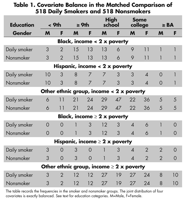
For instance, in both the smoker and nonsmoker groups (in the upper left cells of Table 1), there were three black males with income less than twice poverty who did not complete 9th grade. The five education categories are less than 9th grade, 9th grade or more without a high-school degree or equivalent, high-school or equivalent degree, some college, and at least a BA degree. Indeed, for every pair of cells in Table 1, the counts in smoker and nonsmoker groups are identical, so the joint behavior of these four covariates is perfectly balanced. The perfect balance seen in Table 1 is much better than the balance expected on these four covariates by flipping coins, by complete randomization of individuals to smoking status. Importantly, randomization tends to balance measured and unmeasured covariates, while matching for observed covariates does not typically balance unmeasured covariates. The top two boxplots in Figure 1 depict the balance for the two continuous covariates, namely age and the ratio of income to the poverty level. The matching method that produced this matched comparison forced the balance seen in Table 1 and then made individual pairs as close as possible.
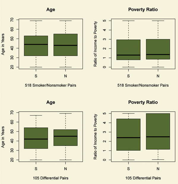
Figure 1. Balance of two continuous covariates, age and ratio of income to the poverty level, for daily smokers (S) and nonsmokers (N). The top boxplots refer the comparison of smokers and nonsmokers; the bottom boxplots to the differential comparison. After matching, the distributions of age and income are similar for daily smokers and nonsmokers.
The matching in Table 1 has already done a great deal of work. Before matching, the measured covariates were substantially different among daily smokers and nonsmokers. For instance, in the complete NHANES data, the odds in favor of nonsmoking rather than daily smoking are 24.4 to 1 for individuals with at least a BA degree and income at least twice the poverty level, but they are 2.2 to 1 for individuals with less than a high-school education and income below twice the poverty level, so the ratio of the odds is 11.4 (with 95% confidence interval [6.9, 18.8]). Despite heavy taxes on cigarettes, in the complete NHANES 2009-2010 data, daily smoking rather than nonsmoking is far more common among people with limited income and education than among people with at least moderate income and a BA degree. This visible bias is removed by the matching in Table 1 and Figure 1, as is its interaction with gender, ethnicity and age, controlling both age and income as continuous variables. Still, there is nothing to ensure that daily smokers and nonsmokers are comparable in ways that we cannot see.
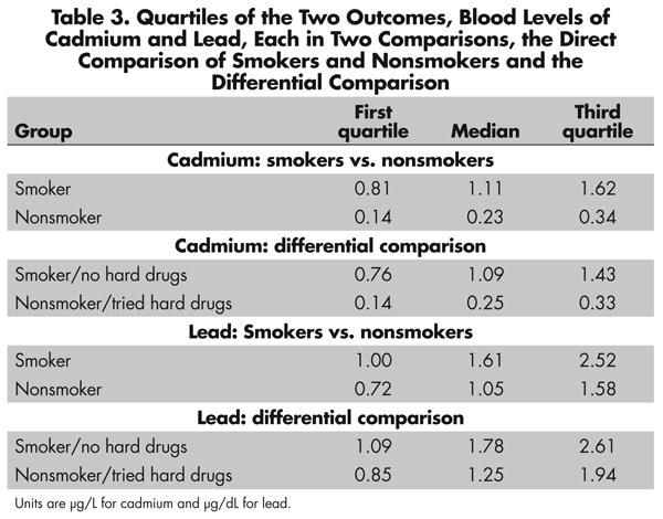
The upper half of Figure 2 compares daily smokers and nonsmokers in terms of two outcomes, two toxins in the blood, namely levels of cadmium and lead. See also Table 3. Tobacco contains both cadmium and lead. Smokers have higher levels of both cadmium and lead in their blood than do nonsmokers. Could fair coin flips produce the pattern in Figure 2? Fair coin flips have a .5 chance of a head, a .5 chance of a tail, or 1-to-1 odds, (1 = .5/.5). A naive analysis that pretended the matched pairs came from a paired randomized experiment would judge the difference in cadmium and lead to be much too large to have been produced by an unlucky sequence of fair coin flips assigning one person in a pair to treatment, the other to control. Indeed, the coin flips would have to be quite biased to explain the difference in lead, at least heads with probability .74, tails with probability 0.26, or odds of 2.9-to-1, a large departure from a randomized experiment. To produce odds of 2.9-to-1, an unmeasured covariate u that increased the odds of daily smoking by a factor of 5 would need also to increase the odds of a positive pair difference in lead by more than a factor of 6. The difference in cadmium is even more resistant to being explained in terms of biased treatment assignment, at least heads with probability 0.98, tails with probability .02, or odds of 64-to-1. So the comparison for lead, and especially the comparison for cadmium, is quite insensitive to bias from an unmeasured covariate. What else can be done to address unmeasured biases?
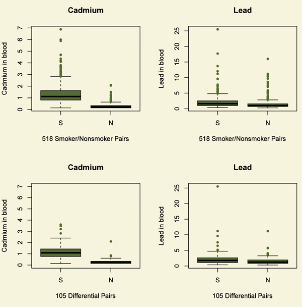
Figure 2. Two outcomes for daily smokers (S) and nonsmokers (N). Blood levels of cadmium are in µg/L, while blood levels of lead are in µg/dL. The top boxplots refer the comparison of smokers and nonsmokers; the bottom boxplots to the differential comparison. Daily smokers have more cadmium and lead in their blood than do matched nonsmokers.

By smoking every day, a daily smoker is expressing a willingness to indulge a habit that can damage health. Perhaps daily smokers do this in more than one way, indulging more than one habit, taking more than one health risk. Indeed, there is evidence of this. NHANES asked, “Have you ever used cocaine, crack cocaine, heroin, or methamphetamine?” Among the 1,036 daily smokers and nonsmokers in Table 1, an answer was obtained from 886 individuals, or 86%. There were slightly, but not significantly, more responses from the daily smokers. Among those who responded, smokers were far more likely to respond “Yes,” the odds ratio being 6.0 (95% confidence interval [4.0, 9.1]). That is, daily smokers were six times more likely than nonsmokers to say they had tried cocaine, crack cocaine, heroin, or methamphetamine (henceforth “hard drugs”).
A strong relationship between smoking and drug use is not a surprise. In particular, cocaine and methamphetamine are stimulants, and it is not surprising to find that people fond of one stimulant are fond of others as well, such as nicotine in tobacco, or caffeine in coffee or tea. One could adjust for hard drugs as an additional covariate, but that would take account of just one coarse measure of one more hazardous habit. The differential comparison in the next section tries to address not one more hazardous habit, but rather a general willingness to indulge bad habits, a willingness partially expressed through daily smoking; partially expressed through use of cocaine, crack cocaine, heroin, or methamphetamine; and partially expressed in other habits not measured in NHANES.
The Differential Comparison: Lifelong Nonsmokers with a Checkered Past
Although daily smokers were six times more likely than nonsmokers to have used hard drugs, there are plenty of daily smokers who never used hard drugs, and there are some nonsmokers who have used them. In the previous section, the smoker group has an excess of people who have used hard drugs and the nonsmoker group has a deficit. The differential comparison removes, for one analysis, the people who did both and the people who did neither, that is, the daily smokers who used hard drugs and the nonsmokers who never used them. The differential comparison compares daily smokers who never used hard drugs to nonsmokers who have used them. The differential comparison does not compare daily smokers and nonsmokers who look similar; rather, it overcompensates, comparing daily smokers who indulge one unhealthy habit to lifelong nonsmokers who have indulged a different unhealthy habit.
As indicated in the sidebars and the Further Reading, the differential comparison can be unbiased by an unmeasured covariate u when a comparison involving either smoking or hard drugs alone would be severely biased by u. This would occur if u promotes both unhealthy indulgences in a similar way.
Obviously, as mentioned before, the differential comparison, even if unbiased, estimates the effect of daily smoking in lieu of having used hard drugs, not the effect of daily smoking. With that firmly in mind, let us look at the differential comparison.
The differential comparison involves 105 matched pairs of a smoker who never used hard drugs and a nonsmoker who has used them. All 105 of these daily smokers were in the treatment/control comparison in the previous section. Only 34 of the nonsmokers who had used hard drugs were in the treatment/control comparison; the remaining 71 nonsmokers were among the unmatched nonsmokers in NHANES. Table 2 and the bottom half of Figure 1 describe the covariate balance in the differential comparison. As in treatment/control comparison, the balance for measured covariates in the differential comparison is quite good.
The bottom half of Figure 2 depicts blood cadmium and lead levels in the differential comparison. See also Table 3. Notably in Figure 2, daily smokers who never used hard drugs have more cadmium and lead in their blood than do lifelong nonsmokers who have used hard drugs. The difference is more dramatic for cadmium than for lead, but the difference for lead is not small. Indeed, comparing the top and bottom of Figure 2, daily smokers who never used hard drugs look quite a bit like daily smokers generally, and lifelong nonsmokers who have used hard drugs look quite a bit like nonsmokers generally.
Although there is a strong association between use of hard drugs and daily smoking-an odds ratio of 6 in treatment/control comparison-a generic tendency to indulge hazardous habits does not explain the high levels of cadmium and lead in the blood of daily smokers. The high levels of cadmium and lead are specific to smokers, not common to people who indulge one of two hazardous habits.
The differential comparison is immune to generic biases, but it is possible that there is an unobserved covariate u that creates a differential bias, promoting daily smoking but not use of hard drugs. To explain the difference in lead in the differential comparison, such a differential bias would need to shift the within pair probabilities from fair at .5-to-.5 for an odds of 1 to .64-to-.36 for an odds of 1.8. Odds of 1.8 could be produced by an unmeasured covariate that more than tripled the odds of daily smoking-without-hard-drugs versus hard-drugs-without-smoking and more than tripled the odds of a positive pair difference in lead levels. A much larger differential bias would need to be present to explain the higher levels of cadmium among daily smokers in the differential comparison, a move from fair assignment at .5-to-.5 for odds of 1 to .96-to-.04 for odds of 23.
As noted repeatedly, the differential comparison, even if unbiased, estimates the effect of daily smoking in lieu of having once used hard drugs, not the effect of daily smoking versus nonsmoking. If we are interested in the effects of one treatment, the most useful differential comparison will be with another treatment that is not known or believed to cause the outcome of interest, but is thought to be biased by some of the same unmeasured covariates. It would not be useful to study the differential effects of heavy smoking and heavy alcohol consumption on blood lead levels because both treatments are thought to increase blood lead levels, so both might have substantial effects yet zero differential effect; however, this might be a reasonable comparison for the effects of smoking on blood cadmium levels. In the current example, having once used cocaine, heroin, or methamphetamine marks an individual as willing to take some risks associated with harmful substances, so this treatment holds some promise for a differential comparison.
Similarly, consumption of coffee indicates a fondness for stimulants, yet coffee is not thought to be a source of cadmium or lead, so consumption of coffee also holds some promise for a differential comparison. The same is true for tea. Obviously, one might conduct several differential comparisons in support of one direct comparison.
Evidence Relevant to Unmeasured Biases
Patterns visible in observed data provide evidence relevant to claims about unmeasured biases. We have just seen three such patterns. First, an observed association may be insensitive to unmeasured bias, so only large unmeasured biases from nonrandom treatment assignment could explain the association as not caused by the treatment; see, especially, the discussion of cadmium. Second, a difference in outcomes in a differential comparison cannot be explained by a generic unmeasured bias, one that promotes both treatments in a similarly biased way. Smokers who never used hard drugs were compared to nonsmokers who had used hard drugs, but it was only the smokers who had elevated levels of blood toxins. The result of this differential comparison cannot be explained by an unmeasured covariate associated in a similar way with both daily smoking and having tried hard drugs. Third, the differential comparison itself may itself be insensitive to a differential unmeasured bias, a bias that promotes only one of the two treatments in the differential comparison. The comparison of daily smokers who never used hard drugs to nonsmokers who used them is, itself, fairly insensitive to the kinds of biases not removed by the differential comparison; see, especially, the discussion of cadmium in the differential comparison.
The differential comparison overcompensates for observable quantities, comparing people who look different, in an effort to compare people who are similar in terms of some unmeasured covariate. The differential comparison is a straightforward and often enlightening supplement to a basic analysis that compares people who look similar.
Further Reading
The theory of causal inference in randomized experiments was developed by Sir Ronald Fisher and is the centerpiece of his Design of Experiments. All theoretical assertions made in this essay about differential effects and generic biases are extensively developed in Rosenbaum (2006). For a survey of multivariate matching in observational studies, see Stuart (2010); for a modern application, see Zubizarreta et al. (2013); and for discussion of the design of observational studies, including matching, sensitivity analysis, the power of a sensitivity analysis, and design sensitivity, see Rosenbaum (2010). In particular, the rationale for comparing heavy smokers and nonsmokers is discussed in Rosenbaum (2010, §17.3) and Zubizarreta et al. (2013). There, it is shown that a comparison focused on substantially different doses of treatment is expected to be less sensitive to unmeasured biases. The process of interpreting a one-parameter sensitivity analysis in terms of two parameters-a so called “amplification”-was illustrated several times here, and is illustrated with more detail in Zubizarreta et al. (2013, p. 85), where further technical references (e.g., ref. 34) may be found. The matching method used here combined minimum distance matching with fine balance for the covariates in tables 1 and 2; see Rosenbaum (2010, §10).
There is an extensive literature on cadmium and lead from smoking; see, for instance, Shaper et al. (1982). Whether the levels of lead visible in Figure 2 are safe levels is the topic of current debate; see Menke et al. (2006) for an empirically based claim that lead at these levels is unsafe.
Several packages in R perform tasks illustrated here. Multivariate matching is performed by Ben Hansen’s optmatch package, Dan Yang’s finebalance package, and José Zubizarreta’s mipmatch package (which requires CPLEX and hence is not at CRAN; therefore, google mipmatch). Luke Keele’s rbounds package performs sensitivity analysis associated with Wilcoxon’s signed rank test and related methods, while Dylan Small’s Package Sensitivity CaseControl contains a function, adaptive.noether.brown, that implements a sensitivity analysis for a powerful adaptive version of Bruce Brown’s combined quantile average test. Ruth Heller’s crossmatch package provides a useful check for multivariate covariate balance in matched pairs. Software aids for matching (and alas errata) in Rosenbaum (2010) are available at my web page www-stat.wharton.upenn.edu/~rosenbap/index.html.
Fisher, R.A. 1935. Design of experiments. Edinburgh: Oliver & Boyd.
Menke, A., P. Muntner, V. Batuman, E.K. Silbergeld, and E. Guallar. 2006. Blood lead below 0.48 micromol/L (10 microg/dL) and mortality among US adults. Circulation 114:1388-1394.
Rosenbaum, P.R. 2006. Differential effects and generic biases in observational studies. Biometrika 93:573-586.
Rosenbaum, P.R. 2010. Design of observational studies. New York: Springer.
Shaper, A.G., S.J. Pocock, M. Walker, C.J. Wale, B. Clayton, H.T. Delves, and L. Hinks. 1982. Effects of alcohol and smoking on blood lead in middle-aged British men. British Medical Journal 284:299-302.
Stuart, E.A. 2010. Matching methods for causal inference. Statistical Science 25:1-21.
Zubizarreta, J.R., M. Cerdá, and P.R. Rosenbaum. 2013. Effect of the 2010 Chilean earthquake on posttraumatic stress: Reducing sensitivity to unmeasured bias through study design. Epidemiology 24:79-87.
About the Author
Paul R. Rosenbaum is the Robert G. Putzel Professor in the department of statistics at the Wharton School of the University of Pennsylvania and a senior fellow of the Leonard Davis Institute of Health Economics at the University of Pennsylvania. He is the author of Observational Studies (2nd edition 2002) and Design of Observational Studies (2010), both published in the Springer Series in Statistics.
Editor’s Note: This article was supported by NSF grant SES-1260782.


