
Mommy’s Baby, Daddy’s Maybe: A Closer Look at Regression to the Mean

Regression analysis is one of the most useful techniques we have in statistics, and it is applied in a large number of disparate situations. It is used to explain the influence (independent) variables have on the variability of (outcome) variables, and this serves us well not only in explaining variability, but also in projecting the future.
The label “regression” survives, but its backward connotation is too narrow to properly describe how the technique is used today. In fact, the name, coined by Francis Galton in his study of eugenics, came about much later than the introduction of the method. Galton was trying to explain data that showed offspring of tall parents were, on the average, not as tall as their parents, and, at the same time, the offspring of short parents were, on the average, not as short as their parents, even though the generational average remained the same. This phenomenon, where the offspring might be viewed as tending toward a population average, is presently referred to as regression toward the mean, although it was originally called regression to mediocrity. This latter label is possibly more reflective of the tenor of eugenics and the subsequent damage it wrought.
Galton provided a detailed explanation of this phenomenon in his 1886 publication, and it was later exemplified by a study that was the subject of 1903’s influential paper, “On the Laws of Inheritance in Man: I. Inheritance of Physical Characters,” by Karl Pearson and Alice Lee.
One problem Pearson and Lee had with their analyses was that their numbers seemed incongruous with the notion that both parents were equally responsible for the height of their offspring. The coefficients of the mother’s height in the regression equations they calculated were invariably higher than the father’s coefficients, and they attributed this to the fact that women were shorter than men.
Galton had run into this same inequality earlier. With his background being in genetic experiments with sweet peas, where it was thought cross-fertilization did not take place, he had to decide how to handle the influence of two parents. To overcome the problem, Galton had simply multiplied the heights of the mothers by 1.08 (based on the ratio of the mean male height and the mean female height), and then averaged the parents’ heights to obtain the mid-parent height. Another way of viewing this is that the father’s height counts for 48% and the mother’s height counts for 52% of the average, and thus the mother is more important.
The Pearson and Lee paper plays a singular role in the folklore of statistics, if not in the history of statistics. So, it is interesting to search for a simple explanation for the behavior of their data. Admitting the mother’s measurements are more important than the father’s when predicting the height of an offspring may mean one of two things: The mother is more biologically important than the father or the mother’s height is more accurately measured than the father’s.
We argue that the latter is plausible; indeed, more than likely, if one acknowledges a human behavior that is probably as old as marriage itself—marital infidelity.
Before expanding on our alternative explanation, we review some of the results contained in the Pearson and Lee paper. The respondents in the study (many of whom were students who probably would not have been made aware of the actual parentage of the offspring, even if they had had the temerity to inquire) were asked to measure family members’ stature (the name Galton used for height), arm span, and forearm. After some explanations by Pearson, the students chose through a nonetheless ambiguous method a representative son and daughter for each family, when they could, and reported on 1,078 families. In the paper, they also reported on statistical analyses dealing with stature, arm span, and length of forearms, but we focus mainly on what the article had to say about height, since that is the aspect of the paper that has generated the most interest.
Table 1 contains some of the summary statistics for these data. We see that, on the average, the sons are an inch taller than their fathers and the daughters are more than an inch taller than their mothers. At first, this seems a lot to gain in one generation (assuming this could not be attributed to the parents shrinking, but we do not know the age of the parents), and certainly that rate of growth was not sustained throughout the last century or we would all be a lot taller by now. Possibly, this is an indicator of the quality of the data one should keep in mind.

That observation notwithstanding, we also can report the correlation coefficients they calculated between the four groups of individuals, done in Table 2. Subsequent to these calculations, the authors fit various regressions, and Table 3 shows those they report for height.

The most often-quoted equation is probably Equation (1) in Table 3, evaluated at some fathers’ heights. For example, the sons of fathers 64” tall average about 67”, and the sons of fathers 72” tall average about 71”. Here, we see the genesis of the label regression to the mean.

There is an intriguing footnote to Equation (2) in Table 3 in the Pearson and Lee article: “If Father and Mother are to contribute indifferently to Son’s stature, the parental statures should be in the ratio of about 560 to 516, which is very nearly the ratio of 1.085 to 1 and almost exactly equal to the 1.083 to 1 ratio of Father’s to Mother’s average stature.”
Why they chose to place this footnote where they did is a mystery. If they had based their comparison on Equation (3), which would seem to be the logical choice given there are two parents to every child, the ratio in question would be 1.051, an awkward number for them to explain.
This is probably what Freedman et al. explain away in their 1991 Statistics textbook by reporting Equation (3) in Table 3 as approximately
![]()
The reason for writing it this way is to get it in a form that uses the mid-parent height. The mother’s coefficient of 1.08, instead of the expected 1 demanded by the mid-parent height formulation, (Galton notwithstanding) is explained away as an adjustment to “women’s heights, increasing them by around 8% so they are just as tall as men.”
This rationalization is a little too facile. The regression coefficients in the linear regressions shown here are not affected by the averages of the covariates, except for the constant term—compare the constant terms in equations (1), (2), and (3) with those in equations (4), (5), and (6), for example. In other words, the 1.08 would be 1.08 whether the mothers were one foot taller or shorter; it is independent of the average height of the mothers. What it does seem to say, though, is that the reported mother’s height is more important than the reported father’s height when predicting the height of the offspring.
To pursue this thought further, in all the regressions quoted in the paper—the six in Table 3 and the corresponding six for span not reported here, plus the six for forearm, which are also not reported here—the regression coefficient for the mother is higher than the corresponding one for the father.
This phenomenon is too regular for us to pass off as women tending to be shorter than men. But supposing that explanation is correct, then the ratio of the coefficients (mother to father) should also be 1.08 in the daughters’ regressions, which it is not. The ratio is 1.12 when comparing equations (4) and (5) and 1.12 when comparing the coefficients in Equation (6). So the previous 8% factor by which we needed to increase the mother’s heights when dealing with the sons, has now increased by 50%, to 12%, when considering the daughters, rather than the sons. This is incongruous, especially since the daughters are shorter than the sons.
As mentioned earlier, Galton ran into similar discrepancies in his analysis. While his raw data has been made publicly available (including a recent electronic version by J. A. Hanley), we posit an explanation for the discordance using the summary statistics from Pearson and Lee (1903). The values from both sources are similar; however, those of Pearson and Lee are based on a data set with approximately five times the number of families used by Galton.
An Errors-in-Variable Model
Our explanation of the discrepancy involves use of an errors-in-variable model. Consider the simple regression for j = 1, . . . , n,
![]() (7)
(7)
where the εj are independent and identically, normally distributed with mean zero and variance σ2e . Suppose the covariate m is observed correctly, but that f is possibly measured with error: instead of observing f correctly every time, we observe it correctly a proportion (1 − p) of the time, and we observe it incorrectly a proportion p of the time. So, for j = 1, . . . , n we actually observe
To estimate the parameters of such models, we need to look to the literature on errors-in-variables (see L. J. Gleser’s 1992 Journal of the American Statistical Association article, “The Importance of Assessing Measurement Reliability in Multivariate Regression,” for example) and specify the model more precisely.
Consider the model where y represents the height of the son (or daughter), m represents the height of the mother, and f represents the height of the father. With apologies to the Latin poet who wrote mater semper, pater numquam, certus est, p then represents the probability that the reported father is not the biological father, and, in those cases, c is the height of the biological father. We need to specify something about the distribution of c and the value of p.
As a working hypothesis, we can take the distribution of c to be equal to that of f, and assume both of them to be normally distributed. The plausibility of the equality of these two variables is supported first by the reported fathers and sons having approximately equal standard deviations of 2.70 inches and 2.71 inches, respectively, and second by arguing that the next generation of biological fathers and reported fathers is part of this generation’s sons.
Further, we assume the heights of the reported and biological fathers are independent, when they are not the same person. We also need to make an assumption about the covariance between the mother’s height and the biological father’s height. Two extremes present themselves: first, that the covariance is the same as that between the mother and the reported father, and second, that the covariance is zero. A third extreme would have the covariance be the negative of the covariance between the mother and reported father, but we do not consider this possibility.
Using the convention that σ refers to the covariance between its two subscripts, we introduce a to indicate the two possible covariances we entertain between m and c:
Thus, in our notation, Pearson and Lee fit the model
![]()
by ordinary least squares, and obtained the estimates in equations (3) and (6). But these values  are consistent estimators of the attenuated parameters:
 (8)
(8)
where the matrix Λ is
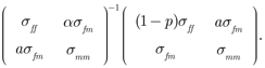
We refer to the matrix Λ as the attenuation or reliability matrix. Note that Λ is the identity matrix if p = 0.
Equation (8) points the way to consistent estimators for βm and βf ; namely, one replaces β by component estimates obtained by using consistent estimators and solves the resultant expression for βf and βm. These are the estimators we calculate below, once we decide p.
Determining the value of p is problematic. The topic is taboo, and this adversely affects our ability to estimate p with any accuracy. This does not imply that we should ignore the issue, and, like Pearson and Lee, use the unrealistic value of zero for p, since this action yields biased estimators. These, in turn, lead to the need for some tortured explanations, as evidenced in their writings.
In their 1991 Lancet article, Macintyre and Sooman remarked that students in British medical schools are taught that p is 10–15%, genetics textbooks report 10%, and even higher numbers have been reported for some parts of England. It is important to note that these numbers are anecdotal and not based on documented studies. What makes it even more difficult, of course, is that we need to project our thoughts back a century. But one can still map out the effect of p, as we show numerically in Table 4 and graphically in Figure 1, where we list some of the results for various ps.
In both Table 4 and Figure 1 we see that recognizing p is not zero increases the estimate of the father’s coefficient in each of the four columns. The value of p needed to attain equality of the contributions of the two parents depends on a. If a = 1, meaning that σcm = σfm, then in the case of the sons’ regression, the p needs to be about .035, in which case the coefficient estimate is .425. For the daughters’ regression, p needs to be slightly higher at .075. And in this case, the coefficient estimate is .420. It is rather surprising that these two sets of regression coefficients are essentially the same, even with different ps.

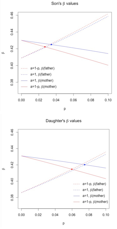
Figure 1. A graphical representation of Table 4, where we have plotted p versus β, for the sons and daughters. The value of p needed to attain equality of the contributions of the two parents is the intersection of same-colored lines.
That the ps are different is not bothersome since some families had no daughters and some had no sons, and so different data were used in the two sets of regressions. Of course, the difference need not be explained away solely on this ground, since we also must remember that a reported brother and sister do not necessarily have both parents in common.
Another set of results is obtained when a = (1 − p), or, equivalently, when σcm = 0. In this case, a p of .027 is needed in the sons’ regression to yield a common regression coefficient estimate of .422. For the daughters’ regression, p must be .060, and this results in a regression coefficient for the parents of .415. A lower p than in the previous situation, but, once again, a close agreement between these two regressions.
Discussion
The constancy of the common regression coefficient (of approximately .42) across all four regressions is consistent with the theory that each parent contributes equally to an offspring’s height. This stands in contrast to the variability evident in the coefficients calculated by Pearson and Lee (equations (3) and (6) in Table 3), which were based on a model that assumed the reported father and biological father were, in all cases, the same man. Our common regression coefficient means both scenarios considered yield parallel regressions for daughters’ heights and sons’ heights when regressed onto parents’ heights. Letting p represent the probability that the father’s height is measured incorrectly, or equivalently, letting p represent the probability that the reported father is not the biological father, our results also seem to lend further credibility to the hypothesis that p is not zero. The values of p required to attain this equality are well within the range of values of available estimates. What is surprising is that small values of p can have such a qualitative effect on the results.
The choice of covariance between the mothers’ heights and the biological fathers’ heights seems to have influence on the p that it takes to achieve equality in the parent regression coefficients. Here, we considered two possibilities: when the covariance between the mothers’ heights and the biological fathers’ heights is the same as the covariance between the mothers’ heights and the reported fathers’ heights (a = 1), and when the covariance between the mothers’ heights and the biological fathers’ heights is 0 (a = 1 − p). However, the covariance specification does not seem to affect the value of the regression coefficient estimates much. One can be quite creative with the assumption about this covariance. For example, the tall, dark, and handsome stranger of the novels of the period jump to mind as a means of providing an explanation for the inch the sons have on the fathers and the 1.35” the daughters have on the mothers. On the other hand, if the biological father was sought to overcome an infertility problem, then presumably his resemblance to the reported father might be a factor that influences his being chosen. Unfortunately, as already mentioned, this subject is taboo, even to this day, so it is impossible to find support or refutation in the literature for a complete consort theory.
We have treated the requirement that each parent contributes equally to the height of their offspring to mean the equality of the two parents’ coefficients in regression equations. Alternatively, one might argue that the four correlations between son and mother, son and father, daughter and mother, and daughter and father are all essentially equal, and that this might be taken indirectly as a satisfactory fulfillment of the equal contribution requirement. Of course, these correlations reflect marginal relationships and the regression coefficients reflect joint relationships, this latter characteristic being more satisfying because it takes into account simultaneously the effect of both parents.
With the Pearson and Lee models, we must choose one or the other, correlations or regression coefficients. Using least squares, it can be shown that this is because the mother’s standard deviation is smaller than the father’s (Table 1), precluding equality of the mothers’ and fathers’ coefficients when regressing either sons’ or daughters’ heights on parental heights (Models (3) and (6) in Table 3). In contrast, the errors-in-variable model does not force us into this choice and gives us equality in both domains—the correlations in Table 2 and the regression coefficients in Table 4.
Furthermore, throughout this analysis, we have taken the mothers to be known. This may not be quite correct. In 1988, Kimberly Mays Twigg was discovered to have been switched at birth in a Florida hospital almost 10 years prior and raised by an unknowing couple. This case establishes, in the United States at least, that a baby can be switched at birth even today. However, in general, the probability that the reported mother is the biological mother should be close to one.
It should go without saying that a good plant or animal genetic study requires that the scientists keep careful records of the parentage. Unfortunately, this principle did not lead to the identification of human parentage in eugenic studies. The investigators seemed to rely on what was reported by the families being interviewed. Possibly Galton or Pearson and Lee considered that as a result of how the data were gathered, the mother’s measurements were more important than the reported father’s measurements, but this consideration is not reflected in their analyses. It is true that regression analysis was still in its infancy at the turn of the century, but in 1877, R. J. Adcock had already published on the subject of measurement error in the independent variable, as had C. H. Kummell in 1879. In 1901 Pearson, himself, suggested the same estimator as Adcock.
The model used in this paper is a mixture model, which is different from the linear errors-in-variables models familiar at that time (Pearson, for example, considered the situation of the linear model with the independent and outcome variable both measured with the same error variance). But the techniques used in the current paper rely on the method of moments, which, of course, was well known to Pearson (as described by Stigler in his 1986 book on the history of statistics). So it seems like the original analyses performed by Pearson and Lee were confined by social norms, rather than any shortcomings in the breadth of techniques available at the time.
Further Reading
Galton, F. 1886. Regression towards mediocrity in hereditary stature. Journal of the Anthropological Institute 15:246–263.
Gleser, L.J. 1992. The importance of assessing measurement reliability in multivariate regression. Journal of the American Statistical Association 87(419):696–707.
Pearson, K., and A. Lee. 1903. On the laws of inheritance in man. I. Inheritance of physical characters. Biometrika 2(4):357–462.
About the Authors
Marcello Pagano is professor of statistical computing in the department of biostatistics at the Harvard School of Public Health.
Sarah Anoke is a doctoral student in the department of biostatistics at the Harvard School of Public Health.


