
Searching for the Black Box: Misconceptions of Linearity

You have lost contact with an unmanned surveillance plane as it is flying over a large stretch of uninhabited desert. You send high-altitude reconnaissance aircraft to take pictures of a potential crash site in the middle of the desert. The pictures reveal large pieces of what you believe are debris from the crashed aircraft. You hope to find the flight data recorder to gain some clues to what caused the crash. Unfortunately, the flight data recorder is too small to be seen in the pictures. You believe that the flight recorder must be present somewhere within the debris field of larger, visible aircraft fragments.
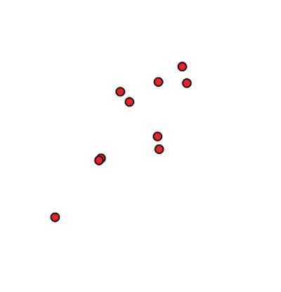
Figure 1. A sample debris field.
Before incurring the costs of a ground force search team, you hope that the debris field can help you predict reasonable potential locations for the recorder. Using the locations of the pieces, you wish to find the best line of flight of the plane so you can search along that direction to find the recorder.
You have to address these questions:
- What criterion should be used to find the best line of flight?
- Does the fact that there is no natural rectangular coordinate system for this situation affect the method to be used to determine this line or our answer?
Early on, statistics students are introduced to fitting a line to a scatterplot of bivariate data and making predictions from such information. The standard assumption is that the x-values are exact, while there may be errors in the y-values or observed data. As characterized in Figure 2, the least squares regression line is calculated to minimize the sum of the squared vertical residuals. Enumerating the accuracy of the predictions involves calculating and analyzing the value of R2, or the line’s coefficient of determination. This regression line can then be used to predict the location of additional missing data.
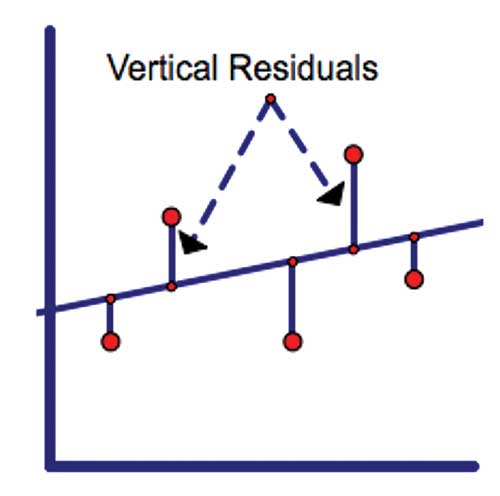
Figure 2. A least squares regression line minimizes the sum of the squared vertical residuals.
For this problem, using a least squares regression line to approximate the line of flight of the aircraft would mean having to decide on a coordinate system to compute the vertical residuals. How should you choose the coordinate system?
You could use the centroid of the data as the origin of your coordinate system or you could choose an origin so all of your data are in the first quadrant. However, computing the centroid requires a coordinate system, and it is not clear that having your data in any one particular quadrant is of any significant value.
How do you orient the data to a coordinate system? The three scatterplots in Figure 3 provide some options for the orientation of the data and, thereby, the coordinate axes.
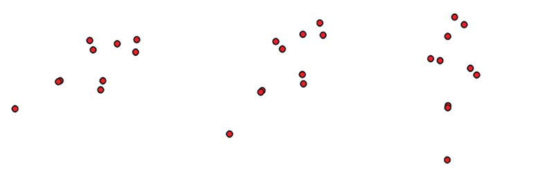
Figure 3. The same data set plotted in three rotational orientations.
Notably, each choice for the coordinate system would produce a different regression line and slope to represent the data. If the scaling (stretching or compressing the data horizontally or vertically) remains consistent among the optional coordinate systems, each choice for a coordinate system can be recognized as either a rotation of the data or a rotation of the coordinate system.
Clearly, this rotation would generate different least squares regression lines. However, the question arises of what is the effect on the least squares regression line and the corresponding value of R2 if the data (or coordinate system) are rotated. Are there rotations of the data that would let you to find the flight recorder more efficiently than others?
This article uses the context of the crashed aircraft to investigate and address common ideas and misconceptions regarding R2; the use of the least squares regression line as the line that best fits a set of data; and an alternative to the least squares regression line as a line of best fit.
Interpretation of R2
In Statistics, McClave and Dietrich say that R2 “represents the proportion of the total sample variability around the mean that is explained by the linear relationship between x and y.” While this interpretation makes sense to a person experienced with statistics, it may not be useful for many others. Let us consider other published interpretations.
Interpretations of R2, the square of the Pearson correlation coefficient r, and r are interconnected. Algebra 1: A Common Core Math Program—Teacher’s Implementation Guide, the Carnegie Middle School curriculum, says, “The correlation coefficient indicates how close the data are to forming a straight line. The variable r is used to represent this value. The closer the r value gets to 0[,] the less of a linear relationship there is among the data points.”
According to Boundless Statistics, “The size of the correlation r indicates the strength of the linear relationship between x and y. Values of r close to -1 or to +1 indicate a stronger linear relationship between x and y. If r = 0, there is absolutely no linear relationship between x and y (no linear correlation).”
The Tutorvista website states, “As R2 gets close to 1, the Y data values get close to the regression line. As R2 gets close to 0, the Y data values get further from the regression line.”
From these descriptions, it is commonly interpreted that if R2 is close to 1, there is a strong linear relationship between the two variables, and if R2 is close to 0, usually one of two situations has occurred: Either the two variables are independent or the relationship between the variables is nonlinear.
It can be inferred from these perspectives that one could use the value of R2 to determine how close the data set is to being along a line, or the linearity of the data. However, in attempting to communicate mathematical ideas to their respective audiences, most of these sources may have inadvertently introduced a misconception about the notion of R2. Before addressing this misconception, we consider the calculations of R2 more deeply and then return to our problem of the line of flight of the aircraft.
Calculating R2 and Its Invariant Transformations
Consider the linear regression model y = β0 + β1x + ε. For the given data points (xi, yi), the mean of the y-values is denoted y. We compute the sum of squares of deviations from the mean using SSyy = Σ (yi – y)2. If ŷi are the predicted values at xi from the linear regression line, then the sum of squares of the errors (deviations) from the regression line is defined as SSE = Σ (yi – ŷi)2.
Let
![]()
Thus, R2 denotes the percentage change in the sum of squares of the deviations that can be attributed to using the least squares line instead of y as a predictor.
A second representation of R2 is as the square of r—the Pearson’s correlation coefficient. This is given by,

where sx and sy are the standard deviations of x and y, respectively.
Invariance is a mathematical property of objects that remain unchanged under particular transformations. Linear functions remain linear under translations, scalings, and rotations. Similarly, we observe that the value of R2 remains unchanged under the following conditions: (a) translation or rescaling of either the independent or dependent variables; (b) switching the x and y coordinates (logically equivalent to reflecting the data points through the line y = x); and (c) rotating the data about the origin by 90˚.
From the correlation formula, condition (a) holds for r as well as R2. Statements (b) and (c) are similar, since reflecting the data points through y = x switches the x and y coordinates, while rotating through an angle of 90˚ switches the x and y coordinates and negates the new x-coordinate. While switching the data points will change the regression lines, the value of r and R2 will remain unchanged due to the symmetry of the correlation formula. For the moment, the question remains as to whether R2 is invariant over rotations of the data other than rotations of multiples of 90˚.
Finding the Flight Recorder
For our problem, you have to locate the flight recorder for the crashed aircraft. You align the debris field according to three coordinate systems, as seen in Figure 4. Each respective scatter plot reflects the graph of the least squares regression line, the slope of the line, and the associated R2 value.
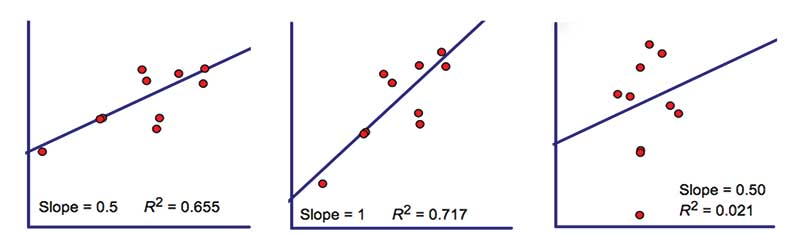
Figure 4. Three coordinate systems with least squares regression lines.
You notice that in the first two cases, the regression line appears to be a reasonably good line of fit to the data, with an adequate R2 value. Both regression lines seem to be usable predictors of the plane’s line of flight. However, you become curious about the third case. You notice that the regression line may not adequately represent the trend of the data and that the R2 value is significantly lower than in the previous two cases.
You suspect that this regression line is not usable in predicting the flight path of the plane. Since all of these scatterplots are simply a rotation of the data or the coordinate system, you find it curious that the regression line no longer follows the data. You begin to wonder why and when the rotation of the data leads to such different linear regressions. You ponder, “If R2 is the measure of the linearity of the data and, in all these cases, the data is no more or less linear (simply rotated), how can this be?”
You begin to believe that the regression line departs from representing the data when the trend of the data gets too steep. You begin to suspect that R2 is not invariant under different coordinate systems (or rotations of the data). Therefore, from the perspective of the least squares regression line and its respective R2, you need more clues to inform your decision about which coordinate system you should choose to find the aircraft’s flight recorder.
As noted, some publications imply that R2 is a measure of the linearity of the data. If so, the scatterplot associated with the greatest R2 value (i.e., the middle scatterplot) may seem most appropriate.
Finding the rotation that maximizes the R2 value may seem like a challenge, but there is a bigger problem. In each of the scatterplots, the data has the same shape and, therefore, precisely the same linearity, yet the regression line and the value of R2</sup varies among each of the rotations of the data. Thus, a contradiction arises: R2 cannot be the measure of the linearity of the data.
To investigate this more deeply, you run a simulation. This simulation rotates a set of data and calculates the least squares regression line and R2 value of the regression line as a function of the rotation. From this simulation, more understanding can be gleaned regarding the relationship between rotations and the value of R2, leading to some recommendations for locating the flight data recorder.
The Relationship Between R2 and Rotation Angle
This simulation involves creating a set of 10 data points that are somewhat close to linear. We take random x-values between 0 and 10, and compute y-values by adding a small random component to the x-values. This produces a set of data that is a perturbation of points away from the line y = x. In the case of the data shown in Figure 1, the points are:
[7.225523 4.293215], [5.176515 3.910213],
[5.901430 6.252120], [3.679196 1.971611],
[8.011683 7.109563], [8.167551 6.546204],
[6.213155 5.904010], [5.244353 3.981286],
[7.410108 6.712347], [7.198705 6.587050].
The simulation rotates the data about the origin and computes the least squares regression line and corresponding value of R2 for each rotation angle. In Figure 5, the resulting slope of the regression line and R2 value are plotted versus the rotation angle. Because of magnitude differences, the scale for each plot is different, as noted on the left and right vertical axes. Notice the 90˚ periodicity in the R2 graph, a property mentioned earlier.
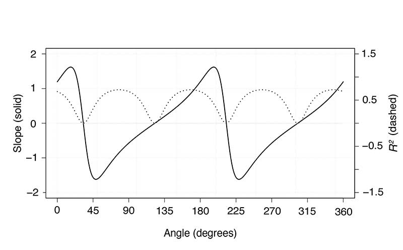
Figure 5. Slope of regression line and R2 as a function of angle of rotation.
The original data have a regression line of slope = 1.00 and R2 = 0.717 (Figure 3, second plot). As rotation angle increases, the slope of the regression line also changes, but in a possibly unanticipated way. The slope increases to a maximum of approximately 1.6, diminishes rather quickly to a minimum of approximately -1.6, and then slowly increases again to the same maximum. Notably, the regression line becomes positively steeper, slows in its increase, reaches its maximum (at approximately 22˚), begins to flatten out, reaches horizontal (at approximately 30˚), passes horizontal and becomes negative, reaches its negative minimum (at approximately 48˚), and then returns more slowly from negative to its maximum positive slope. This behavior is also cyclic, with a period of 180˚.
Simultaneously, the R2 value of the regression line changes throughout the rotations of the simulation. As the trend of the data rotates to become more vertical, the R2 value of the regression line decreases to almost 0 (at approximately 35˚). As the trend of the data rotates past vertical, although the slope of the trend line of the data is now negative, R2 increases to 0.717 until it begins to again diminish (at approximately 75˚). This behavior is cyclic with a period of 90˚. The angles where R2 is small are the same angles where the data trend line is quite steep and the regression line is mostly horizontal.
Connecting the two graphs, it can be seen that the minimum values on the graph of R2 are where the slope of the regression line is close to 0. Moreover, these points of intersection are at, or near, points of inflection on the graph of the slope of the regression line. Summarily, the linear regression line is a poor representation of the linear nature of the data if the trend of the data is too steep.
A similar effect can be seen in the R2 plot. While the linear-ness of our data remains the same through the rotations, neither the regression line nor the value of R2 remains consistent.
A Better Line of Fit?
Contrary to some resources, the R2 value from a linear regression does not give a measure of the linearity of a set of data, nor does it really provide a measure of goodness of fit (which is really the same thing). The R2 value is only a measure of the correlation between the two variables in the data, which measures how well one variable is reflected in the other. Although correlation is an important statistical concept in the relationship between variables, perhaps R2 is a convenient measure that has been applied beyond its appropriate use.
If you stop here, realizing that R2 does not report the linearity of the data, you may be discouraged in your search for the plane’s flight data recorder. You may opt to employ the coordinate orientation that provides a linear regression with the greatest value for R2. While this may be fine, at least you will do so without being misled by a common misconception. However, perhaps other types of regression lines will follow the trend of the data more consistently, regardless of rotational orientation.
One possibility for a line of fit is the orthogonal regression line, as discussed in Measurement Error Models. Orthogonal regression assumes errors in both variables and minimizes the sum of the squared orthogonal distances from the data points to the line, as shown in Figure 6.
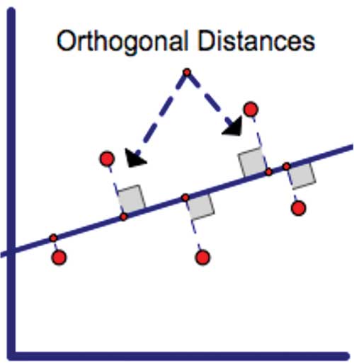
Figure 6. An orthogonal regression minimizes the sum of the squared orthogonal distances.
One promising property of the orthogonal regression line is that it is rotationally invariant (if the data values are rotated by angle θ, then the orthogonal regression line is also rotated b yθ). Unfortunately, the orthogonal regression line does not produce an associated value such as R2 to enumerate the model’s goodness of fit. The plots in Figure 7 show the orthogonal regression line fitted to our three rotated data sets.
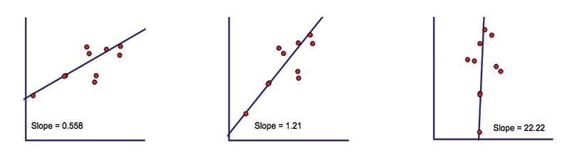
Figure 7. Three coordinate systems with orthogonal regression lines.
You run the previous simulation again. This time, the slope of the least squares regression line, its associated R2, and the slope of the orthogonal regression line are dynamically calculated. This produces the graph in Figure 8.
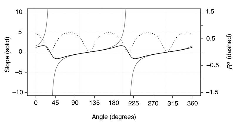
Figure 8. Slope of linear (black) and orthogonal (gray) regression lines and R2 as a function of angle of rotation. Note that the orthogonal regression curve has a vertical asymptote near 30˚ and, therefore, is not continuous.
As the trend of the data becomes more vertical, the orthogonal regression line correspondingly becomes more vertical and its slope tends toward infinity at a value where the linear regression line is close to 0 slope and the value of R2 is minimized. Notably, when the slope of the orthogonal regression line is relatively small (between -2 and 2), the slopes of the orthogonal and linear regressions lines are almost indistinguishable. Thus, the least squares line does a good job of representing the linear trend in the data (despite R2 varying significantly over this range).
However, at a rotation angle range of (30 ± 10)˚, the slopes of the two regression lines are quite different and the orthogonal regression line is far preferable to the least squares regression line.
In summary, there are clearly ranges of rotation in which the linear regression model provides a poor representation of the trend of the data; the orthogonal regression better represents the trend of the data; and the linear and the orthogonal regression lines represent the trend of the data equally well. Therefore, the user should be familiar with both regression lines and be aware of situations in which one line should be preferred over the other.
Conclusion
You return to your task of attempting to predict the location of the flight data recorder and you decide to use an orthogonal regression line in the process. However, your colleagues complain that they would prefer using the least squares regression because the associated R2 value also provides a measure of linearity and would allow them to narrow their search.
“If the R2 value is high,” they argue, “then the data are more linear and we can reduce the width of the search field along the regression line.” You can now respond, “R2 is not a measure of linearity. There are many occasions when another line of fit better represents the trend of the data.”
This scenario is not an isolated case. In many instances, there is either no clear set of coordinates or no clear independent variable, or the measurement error in the independent variable cannot be ignored. In all of these cases, we must take great care when using a standard least squares regression line. We also have to be careful in our use of the R2 value as an indicator of goodness of fit.
We are not suggesting that the orthogonal fit is the solution to all of these issues or that the orthogonal fit is without its own limitations. We merely stress the importance of keeping a clear vision of what a linear regression and its associated R2 value really provide. Perhaps more importantly, we suggest the importance of understanding what a linear regression and its associated R2 value do not provide.
Further Reading
Boundless. 2016. Coefficient of Correlation. Boundless. Retrieved February 24, 2016.
Carnegie Learning, Inc. 2012. Algebra 1: A Common Core Math Program—Teacher’s Implementation Guide (Vol. 2), Pittsburgh, PA: Carnegie Learning Inc.
Fuller, W.A. 1987. Measurement Error Models, New York, NY: John Wiley.
McClave, J.T., Dietrich, F.H., and Sincich, T.L. 1996. Statistics (7th ed.), Upper Saddle River, NJ: Prentice Hall.
Pearson Publishers/Tutorvista. 2016. Coefficient of Determination. Retrieved March 11, 2016.
About the Authors
Michael. J. Bossé is the Distinguished Professor of Mathematics Education and MELT program director at Appalachian State University, Boone, NC. He teaches undergraduate and graduate courses and is active in providing professional development to teachers in North Carolina and around the nation. His research focuses on learning, cognition, and curriculum in K–16 mathematics.
Eric Marland is a professor in the Department of Mathematical Sciences at Appalachian State University and has a broad background in mathematical modeling in the biological sciences. His current research interests lie primarily in carbon accounting methodologies in environmental science and in understanding the role of uncertainty in climate policy.
Gregory Rhoads is an associate professor in the Department of Mathematical Sciences at Appalachian State University. His research interests include applying complex function theory to minimal surfaces and dynamical systems.
Michael Rudziewicz holds a MS degree in mathematics from Appalachian State University and has conducted research on pattern recognition in data.


