Xinping Zhang, Byran J. Smucker, and Jay Woffington

A board member, a marketing professional, and an actor walk into a bar. The actor says, “Why aren’t you spending more money on marketing my great Shakespearean performance?” The board member concurs. “I agree. Why are our sales so slow? Surely, there’s got to be something we can do.” The marketing professional responds, “First, the name ‘Shakespeare’ isn’t helping us here. Second, it’s the most tickets we’ve ever sold to a show like this. Third, stop calling me Shirley.”

At companies and organizations across the country, analytic dashboards give executives and boards of directors a performance snapshots. Dashboards often list sales results, projections, and other key indicators, which are generally compared to this year’s budget as well as totals from the same time last year. Additionally, and with a dashing stroke of creativity, the results might even be color-coded—green for “Everything’s on track,” yellow for “Cautiously optimistic,” and red for “Problem area.” While this shorthand is helpful for time-starved observers who don’t have their fingers on the pulse of the organization, it presumes that the underlying models producing the colors are good or at least adequate. And sometimes, it’s not so easy to know how you are doing.

At the Cincinnati Shakespeare Company (CSC), a professional theater focused on Shakespeare and the classics, more than 25,000 tickets are sold every year for 10 different productions, each with a typical run of 16–20 performances. These ticket sales are the lifeblood of the organization, a small non-profit, and a lot of effort is expended trying to understand how a given show is selling at any point in time. At each staff meeting, the box office manager shares the latest sales data. At each board meeting, the trustees review the dashboard with a specific interest in ticket sales.

But how can you tell if a show, which doesn’t open for a month, will make its goal given its sales to date? Simply put, should it be red, yellow or green? More basically, how do you know if the original goal was even realistic in the first place? Despite having data records for every ticket sale of every performance of every show down to the minute of purchase for the past few years, the organization had no underlying reliable prediction model. The institutional gut had a single metric—“If we hit 20% of our goal before our first performance, we will make the goal.” Not only was this wrong about half the time, if a show failed to meet the rule of thumb there was no time to do anything about it.

A scene from Hamlet. Used with permission by Cincinnati Shakespeare Company.

The CSC’s executive director (and co-author of this article) realized that the theater possessed data that could be used more effectively to give advance notice of possible shortfalls or windfalls. He first enlisted one of his actors, who had some quantitative background, to help improve the predictions. But the ad hoc methods they developed had deficiencies of their own, and so they reached out to Miami University, finally landing in the department of statistics. Over the next year and a half, a more systematic and principled approach was developed and deployed to the CSC in the form of interactive software. In this article, we describe this approach and application.

The value of good predictions is not simply the knowledge itself. The predictions promote better understanding which in turn enables better decisionmaking in the face of uncertainty and limited resources. Should a show be added, or a run extended, to provide additional supply for excellent demand? Should marketing support be increased to prop up sluggish sales, or should the theater simply play out the string and turn its attention to the next production in the queue? Is it going to be so bad that payroll is threatened?

While the choice of red, yellow, or green may not have mattered so much 400 years ago when Shakespeare’s plays were first produced, it is crucial in today’s world. Given the relatively recent development in statistical modeling and information systems, surely (Shirley?) these tools could be leveraged to improve predictions and positively affect the company’s success.

Priming the Data for Action

The raw data collected by the CSC’s ticketing software include the sorts of things one would expect: basic information about each show, patron information, date and time of all purchases, the number of tickets purchased, and the amount paid for them (many of the tickets show an amount of 0 because they are passes issued for season subscribers). The data include complete sales information for 40 shows from the last four seasons (2010/2011 to 2013/2014, which were seasons 17–20 for the CSC). To construct the models we discuss in subsequent sections, we use all the shows in the database and make the simplifying assumption that the total sales of these shows represent independent observations. Because no major changes in, for instance, theater capacity have been realized over the years in question, it seems reasonable to assume that the underlying forces driving ticket sales have remained stable. Figure 1 shows a snapshot of the raw data, with personal data redacted.

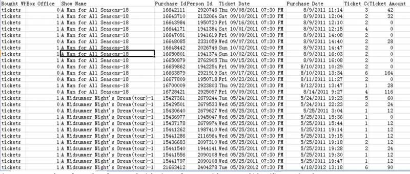
Figure 1. A snapshot of raw data from CSC’s ticketing software, with personal identifiers omitted

The sort of information we aimed to exploit for predictive purposes falls into two broad categories, shown in Table 1: characteristic predictors and sales-related predictors. Characteristic predictors include inherent aspects of a show such as genre and time of year (“Interval” in Table 1; note that if a show straddles multiple categories it is assigned to that category in which it runs the most days). Other characteristic predictors are the number of performances and whether the show has been staged over the time for which we have records (i.e. in seasons 17-20). Genre is a manual classification into four general classes, including “Shakespeare Known” (famous plays such as “A Midsummer Night’s Dream”); “Shakespeare Obscure” (lesser known Shakespearean works such as “Richard II”); “Contemporary Classic” (a play a high school senior would know is not a Shakespeare and whose plot would be somewhat familiar); and “Contemporary” (generally by a 20th-century playwright with a plot unfamiliar to the typical audience member).

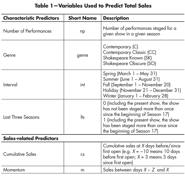
Table 1—Variables Used to Predict Total Sales

The sales-related predictors in Table 1—Cumulative Sales and Momentum—are perhaps the most important. Cumulative Sales is defined as all sales of a given production from the beginning of the sale period through a chosen date X days from first open (i.e. the first staging of the show). Momentum is calculated as the total sales in the Z days preceding. In general, we anticipate that the more cumulative sales at day X, and the greater the momentum, the higher the final sales will be.

To process the data from its raw form (Figure 1) to a structure that can be used to develop a predictive model, we adopt a simple approach: take each complete show in the data set as an independent observation, calculating the total sales for each. To construct the two sales-related predictors, the analyst must specify two quantities, X and Z, based on the sort of predictions he or she would like to make. For instance, if a prediction of total sales is desired based on cumulative ticket sales 10 days before first open and based on the sales (Momentum) over the last three days, then X = −10 and Z = 3. This is illustrated graphically in Figure 2. The CSC is primarily interested in making predictions in the last month or so before the show opens, so X is typically negative, though it could be specified as a positive whole number, representing the cumulative sales X days into a particular show’s run. The momentum, on the other hand, only makes sense as a positive number.

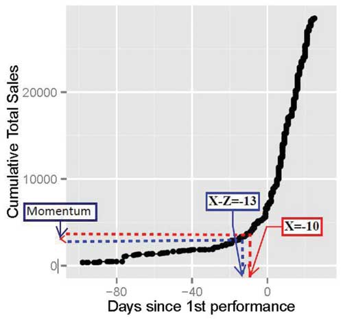
Figure 2. Graphic representation of cumulative sales and momentum for a profile of ticket sales for “A Man for All Seasons,” Season 18 at the Cincinnati Shakespeare Company

Once X and Z are specified, the cumulative sales and momentum predictors can be constructed from the data, and they are used along with the characteristic predictors given in Table 1 to develop a linear regression model (more on the choice of X and Z, as well as model selection, in the next section). This model can then be used to predict the total sales for a future show. This approach also allows the CSC to set an initial goal for sales while deciding which shows to stage for an upcoming season: they can simply use a model that uses only the characteristic predictors.

The general sales profile demonstrated in Figure 2 is typical. There are few sales until several weeks before the show opens, but sales accelerate dramatically in the days leading up to first open.

Constructing a Predictive Model that Makes Good Predictions

Since the CSC runs 10 full shows every season, the models should automatically incorporate new data as they become available. Furthermore, since the theater may wish to make predictions at many different times (i.e. many different values of X) in the lead-up to various shows, the approach should be sufficiently flexible to allow this. For instance, the best model to predict total sales on the day the show opens (i.e. X = 0) using data available in 2015 might be quite different than the best model when a prediction is to be made 30 days (X = −30) in advance of first open using data available in 2018.

Consequently, we use 10-fold cross-validation, in real-time, to select the predictive models. This means that the CSC can use an up-to-date raw data set, and specify X (and Z in some cases), and the software will select an appropriate model and make the desired prediction (more on the software application later). Cross-validation is an approach that allows assessment of a model’s quality in terms of its ability to predict new observations. It proceeds by randomly partitioning the data set into k mutually exclusive sets (folds), holding out a single fold, fitting a model to the remaining k-1 folds, and using the fitted model to predict the held-out data. This process is repeated for each of the k folds. This procedure can also be used to choose a model (following Section 6.5.3 in An Introduction to Statistical Learning with Applications in R by James, Witten, Hastie, and Tibshirani). We considered for possible inclusion in our models all predictors in Table 1, as well as two-predictor interactions not involving Genre or Interval. Those interactions not considered were excluded to keep the models relatively simple, given that Genre and Interval have 4 and 5 categories, respectively.

As intimated above, there are two kinds of models of interest. First, for annual planning purposes the CSC would like a model without the sales predictors (see Table 1). For example, each year during budgeting time, the artistic director chooses a 10-show season.

A key driver of the budget is the ticket projections for each show. Historically, the company would make educated guesses based on general sales trends (“Hey, this year we sold 20% more tickets than last year!”), institutional knowledge (“Audiences loved our last ‘Hamlet.’ We did $35,000.”), and learned heuristics (“History plays in May just don’t sell in this city.”). Using a model based on the characteristic predictors, the CSC can add these predictions to the matrix of inputs that they use to make decisions. Clearly this model will be limited in its capacity to predict, since the characteristic predictors represent only crude information. For the data used in this article, the cross-validation procedure selected a model with just three terms, as can be seen in the “No sales info” row of Table 2. Thus, to predict the total sales of a show, you can use the following equation:

Predicted Total Sales = 23,313 + 2,129 (Number of Performances – 16) + 9,666 (Contemporary Classic) – 5,703 (Number of Performances – 16) (Last Three Years)

where “Contemporary Classic” is 1 if the show is in that genre and 0 otherwise, and “Last Three Years” is 1 if the show has been staged more than once (including the current staging) since the beginning of Season 17. In Table 3 we give predictions for several shows using this and a more complicated model which we describe below.

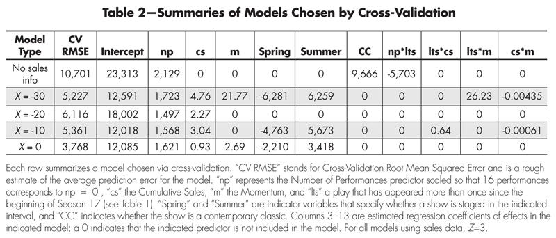
Table 2—Summaries of Models Chosen by Cross-Validation

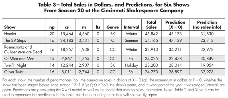
Table 3—Total Sales in Dollars and Predictions for Six Shows from Season 20 at the Cincinnati Shakespeare Company

The second model of interest, for marketing purposes as well as for cash flow management, is one which includes sales predictors to help understand how a given show is selling at any point in time throughout the sale period. The earlier the company can spot a potential shortfall, the more they can influence it with additional marketing spending. Managerially, knowing how a given show is doing at any point in time can help reduce leadership and board concern, or at least manage their expectations and avoid unpleasant surprises.

Figure 3 gives visual results of the cross-validation for several different values of X, chosen as representative of X’s that interest the CSC. (The number of days over which Momentum is calculated has been specified as Z = 3 throughout, based on some initial testing that suggested it performed better than Z = 7. These two values for Z were chosen because of their pleasing intuition; more extensive testing could be performed.) Note that the rough estimate of the average prediction error, “CV RMSE,” is 2–3 times larger for the model that does not use sales data. It is clear that not only does incorporating sales information make predictions better, but also that using sales information as late as the opening day of the show improves the predictions even further. On the other hand, there doesn’t appear to be a great difference between predictions made 10, 20, or 30 days in advance.

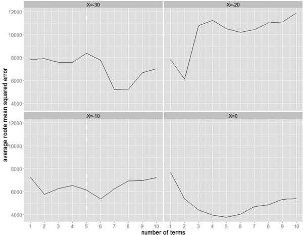
Figure 3. Results of the model selection by 10-fold cross-validation. The y-axis gives a measure of the average error; the x-axis gives the number of terms in the associated model.

The cross-validation procedure explores models with a various number of terms, and looks for the model size that best balances under-fitting and over-fitting, as evidenced by the smallest average root mean squared error. Cross-validation plots, like those in Figure 3, typically have a U-shape, indicating a sweet spot in terms of the number of predictors. Our plots do not uniformly conform to that ideal.

This is somewhat unusual, but may be partially explained by the relatively small number of observations and the categorical nature of some of the predictors. Indeed, when the procedure is run with only the numeric predictors Cumulative Sales, Momentum, and Number of Performances, and their associated two-predictor interactions, the plots are better—though still not perfectly—behaved.

Consider the predictions made by the X = 0 model for shows identified in the data set as Season 20 in Table 3. Overall, they appear quite good and certainly much better than the predictions from the model that does not use sales information. This is not unexpected, given that the average root mean squared error of this model is so much smaller.

What Are the Most Important Predictors?

From Table 2, one can see that the number of performances (“np”) has a reasonably stable relationship with the total sales for the models that incorporate sales information. That is, for the models that use sales information, each additional performance is associated with a roughly $1,500-$1,700 increase in total sales. Furthermore, it is clear that spring shows don’t tend to do as well, and summer shows experience a bump. Anecdotally, the “spring dip” may be due to the many artistic and entertainment alternatives in the region that emerge when the weather breaks, from professional baseball games to end-of-year high school musicals and graduation parties. Similarly, the “summer fling” may be driven by the benefit of being the only theatrical game in town during that part of the year.

For the range of X’s considered, the magnitude of the association between cumulative sales and total sales typically and expectedly declines as we use more recent information. For instance, an increase of one dollar of cumulative sales 20 days out is associated with an increase in total sales of around 2.3 dollars (holding other predictors constant), whereas that factor has shrunk to 90 cents for the X = 0 model. Note that for the X = -30 model, the cumulative sales coefficient (4.8) isn’t quite as large as it appears because also included in this model is an interaction between Cumulative Sales and Momentum. For a show that has a momentum of $279 (roughly the average Momentum when Z = 3), the cumulative sales factor is reduced to 4.8 − 0.0044(279) = 3.6, which is in line with the other models.

Note also that Momentum plays a role in three of the four models that use sales information. For the X = 30 and X = -10 models, the association between momentum and expected total sales is obscured by its involvement in interactions, but by examining the X = 0 model we can interpret this relationship in a straightforward way: That is, every additional dollar in sales in the last three days is associated with an expected $2.7 increase in total sales, assuming all other predictors are held constant.

Toward a Dashboard: A Shiny Application

As described in the introduction, a dashboard is crucial for an organization like the CSC because the primary stakeholders are business and theater professionals, not statisticians. Consequently, unfiltered “regression output” or “R code” will obfuscate rather than clarify. A good underlying predictive model is necessary for the happy melding of analytics and business, but it is not sufficient. The results should be presented in a way that engages and highlights all the results that are important to the organization.

As described above, a significant amount of data reformatting is required to get from the raw database to a form amenable to modeling. The CSC’s limited resources prevented them from hiring someone to build a modeling platform in-house. This necessitated a stand-alone, user-friendly software solution. Accordingly, we used RStudio’s Shiny R package, which facilitates the construction of interactive statistics applications. Behind the scenes, the raw data are processed and combined with user input to produce plots, models, and predictions. The interface displayed in Figure 4 is designed to meet a wide range of needs for those monitoring ticket sales at the CSC. The functions described below are based on the modeling approach described above. That is, linear regression models are chosen via cross-validation and deployed to make predictions in several different ways.

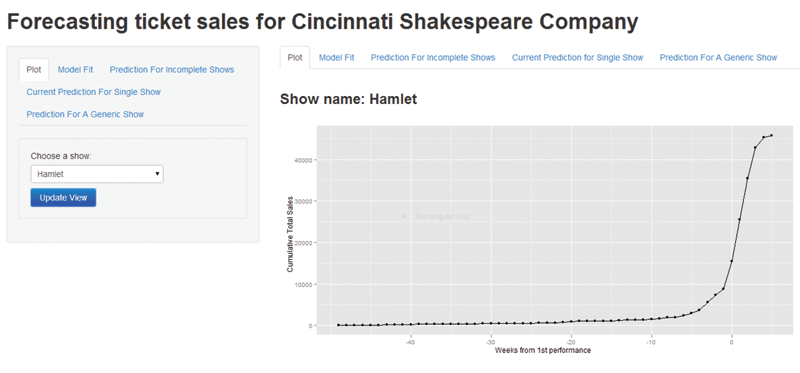
Figure 4. Shiny application user interface

First, any show represented in the database, whether complete or in-progress, can be plotted (e.g. Figure 4). This allows the analyst to quickly visualize the status of a particular show. Second, the analyst can fit a model and see the results for all completed shows. The models can either exclude or include sales information, and in the latter case the type of model that is fit can be controlled by specifying X and Z. This gives an overall view of a model and its predictions for past shows. It can also prompt questions that increase understanding. For instance, a Season 17 production, “Frankenstein: The Modern Prometheus,” is consistently over-predicted by the model. In this particular case, “Frankenstein” was a one-man, off-night show paired with “Dracula,” and likely had less publicity than a typical show. Thus, the lower-than-expected sales are not too surprising.

Third, the program can make predictions for all incomplete shows in the database, based on the last sale date in the database for each show. For instance, in the database used in the development of this application, tickets for “Henry IV” were being sold. Based on the date of the last ticket sale on record, there were still nine days until it opened. Thus, this functionality constructs a model to predict the show’s total sales based on its current sales, its momentum (Z = 3), and the characteristic predictors given in Table 1. This is accomplished, of course, by using X = −9 and constructing a model using all of the completed shows in the database. This part of the program produces sales predictions for all incomplete shows in the current database within 60 days of first open. On the downside, it requires an updated database, which, since it is fairly large, cannot be obtained immediately.

Since the CSC would like to have feedback every day, the fourth function of the program allows the user to choose any show in the database within 60 days of opening and specify its current sales and momentum (Figure 5). Then, based on the current date and the date of the show’s first performance, a prediction will be made. This is perhaps the most important functionality because it does not require an up-to-date database but still allows an up-to-date prediction, as long as the user can specify the current sales and recent sales.

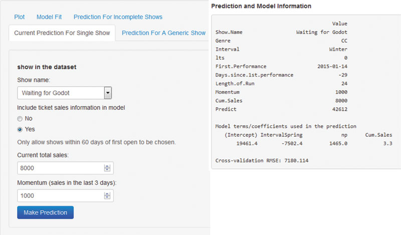
Figure 5. Current prediction for single show (left, input; right, partial output)

Finally, the fifth function of the program is to allow a prediction to be made for a generic show. This show does not have to be found in the database, so this function can be used for planning purposes. It requires the specification of the show’s name, its genre, the time of year it will be staged, the number of anticipated performances, and whether the show has been staged before. This information is enough to allow a prediction, but of course current (or expected) sales data can be used as well. The primary benefit of this function is to allow goals to be made for shows with various characteristics that are being considered for upcoming seasons.

Note that for each of these modeling functions, the analyst can specify whether to include current sales information (Current Sales and Momentum) in the model. For instance, in the “Prediction for Incomplete Shows” function, if current sales information is not used the program will make a prediction of all incomplete shows in the database based only on characteristic predictors.

We note that though the Shiny application was delivered fully functional to the CSC, it has several deficiencies that distinguish it from fully tested, commercial software. For instance, occasionally an error surfaces that prevents the cross-validation procedure from successfully constructing a model. In this case, the user should restart the application to obtain the desired predictions. There are also some quirks in the GUI: for instance, sometimes the output columns wrap around in an unattractive way, and the input and output panels don’t automatically coordinate with each other. Though the CSC indicates that these problems with the GUI are not problematic for their use of the application, newer versions of the application might address these issues.

Summary and Discussion

Information about key performance indicators is important in the operation of any organization, and when information can be exploited to make accurate predictions about the future, it is invaluable. The more effective the models underlying the information and predictions, the more informed, flexible, and empowered the decision-makers are. In this particular case, we have developed least-squares regression models to make predictions to serve a small, non-profit theater in Cincinnati. The models have been deployed to the CSC in the form of a Shiny application, and used by the organization. (See a version of the app here.)

Consider an example of the CSC’s use of these predictive models. In March 2014, there were two shows remaining in the CSC’s season: “Two Noble Kinsmen” (TNK) and “Private Lives” (PL). The question confronting the theater was where to invest their remaining marketing dollars. At the time, the heuristics used in the past, based on a data-less rule of thumb, suggested that TNK was lagging and PL was on track. The model, however, projected that TNK would meet goal while PL was trailing fairly significantly. This caused a shift in the CSC’s thinking, and instead of spending on TNK, they shifted their money to PL. In the end, PL’s momentum was increased and both shows ended up exceeding their goals. This anecdote illustrates how data, as analyzed via a predictive model, have provided insight and altered the behavior of decisionmakers within this organization.

Ultimately, the CSC is interested in two sorts of questions. First, questions about turning data into predictions: How can one set realistic goals for a show in the planning stages? How can one tell at a given point in time whether sales are tracking with the goal or coming up short? Second, there are questions of a more prescriptive nature: Can predictions be used to drive organizational decisionmaking, for instance extending a run if demand is strong or supporting additional marketing to boost lethargic sales? The model developed can directly answer the first kind of question, and allows the CSC to further explore the second.

It is likely that further improvements can be made to these methods. The current procedure doesn’t explicitly use all of the data for each show. That is, once the cumulative sales and momentum, indicated by X and Z, are specified, the construction of the model ignores the rest of each show’s sales profile. It might be better to model these profiles directly. This would, of course, require more complicated statistical methods. One could also imagine other predictors that, if they were available, would probably improve the predictions. For instance, quantifying the advertising for a particular show at a given X, or including an external entertainment index to quantify the entertainment options in Cincinnati at a particular time.

With the model and software described in this article, however, the CSC is now better equipped to make principled predictions, and use them to take appropriate actions. Several times a week, the leadership team hears how the sales are doing for each upcoming show. The dashboard the CSC uses now has an effectively color-coded green each time the model predicts the show will make its goal, yellow when the model shows it slightly under, and red when things look bleak. These cues, even when they are 10, 20, or even 30 days out, are equipping the organization with insight. Now, the actor can know when his presence and performance is inspiring both awe and healthy ticket sales, the board member doesn’t freak out except for a very good reason, and the marketing professional doesn’t spend money on advertising unless the data call for it. And now, they can all walk into the bar and have a celebratory drink as the thinking has made it so.

About the Authors

Xinping Zhang completed her master’s degree in the department of statistics at Miami University in 2013. Much of the work represented in this article was completed as part of her master’s project.

Byran Smucker is an assistant professor in the department of statistics at Miami University. His primary research interests are in the design and analysis of experiments, but he has also consulted on a range of statistical projects.

Jay Woffington is the executive director of the Cincinnati Shakespeare Company, a position held since 2012. Under his leadership the CSC has “completed the canon” by producing all 38 of Shakespeare’s plays. Jay has a master’s degree from Northwestern’s Kellogg Graduate School of Management.

Back to Top