Do We Let Businesses Get away with Dodgy Ethics and Loose Morals? An Application of Markov Random Fields
For a moment, look at the society we form. What’s the glue that binds the key players? The force that keeps the arrangement from collapsing? What makes the entire structure throb? Think awhile, and you’ll realize it’s not the actors but dependence—a reliance among them that makes up the key fabric. Take that dependence away, and people will act chaotically: One’s actions may not be predictive of anyone else’s. It is network science’s job to bring out the apt format of connectedness and use it to summarize societal subtleties, to predict people’s behaviors. Sitting at an intersection of mathematics, statistics, physics, and computer science, out of the specialized data topics we have currently, network science has been attracting probably the steadiest attention over the last decade. Its grandeur and utility explain, in part, its magnetism. Some of that utility will be on fuller display if we, for actors, replace people with less concrete objects like attitudes.
A recent Gallup poll conducted in the United States provides the perfect setting. A group of 5,757 participants across various age groups, political leanings, etc., was asked 128 questions probing how they feel about the way businesses function. Table 1 shows a sample of those questions. Frequently, a major question represented a category, and there were subquestions that tested the participants on subthemes. The 11-series questions, for instance, asked people how crucial they think certain aspects of running a business are; the 12-series questions checked how they felt businesses were actually doing on those corresponding themes. The graphs in Figure 1 represent webs of interconnectedness not among the survey participants—like we’d have on a typical Facebook or Twitter-type social network—but among these attitudes. In a social network, dependence is easy to understand; a link gets formed, (i.e., two people get attached) if they are on each other’s friend lists or if one follows the other. This is a clear binary: at a point in time, you are on someone’s friend list or not—there’s no doubt when or whether a tie is formed. But what makes an attitude “hook up” with another? Varieties of correlations may supply some options.
Let’s Get on to the Field…the Markov Random Field…
One strategy is to check whether certain types of responses from one question always “go with” certain types of responses from another question (much like studying a lot frequently goes with getting good grades) and, in case they do, linking the two attitudes that these questions brought out. This sounds like correlation, but there are two problems: one implementational and the other conceptual. The responses from questions 11 and 12 in Table 1 are not naturally numeric (like hours studied or scores obtained) but on a Likert scale: “not at all;” “not very;” “somewhat;” “extremely;” etc. Ordinary correlations do not bring out the right connection between two such Likert variables—between questions 11A and 12A, for instance. The way out is to assign numbers (1 for “not at all”, 2 for “not very”, etc.) but pretend that there are continuous distributions (typically bell-shaped normals) at the back that gave rise to the 1s and 2s. So, we may assume behind question 11A responses, there is an “importance score” distribution—something we cannot see—a latent or hidden density spanning [0–100], whose lower end corresponds to people who do not think the issue matters at all. For example, someone who feels that increasing profits each year is “extremely” important may have given 94 points out of 100 to this tendency had the response variable been a continuous score. The correlations found from these continuous scores are called polychoric correlations, and through many simulation studies, researchers like Sacha Epskamp and colleagues have found that the polychoric correlations on these Likert data match closely with the ordinary (i.e., Pearson) correlation on the latent data.
The edges in the networks in Figure 1 are made with these polychoric correlations: the blues represent positive correlations, the reds, negatives; the heavier lines represent stronger connections and fainter lines weaker ones. People tend to react similarly to questions 11A and 11B, for instance. Those that say it’s “extremely” important to increase profits each year generally say it’s “extremely” important to meet the financial goals of shareholders and investors. Those two attitudes can, therefore, be good “friends”—they vary similarly. This is how we fix the implementation problem, by choosing the right type of correlation.
Technically, assume two ordinal variables with r and s ordered categories are thought of as realizations from two continuous latent random variables with a joint normal distribution. Then the polychoric correlation is defined to be the solution ρ to
θρ(A1),θρ(A2),…,θρ(Ars) = (ρ1,ρ2,…,ρrs),
where θρ(Ak) is the volume of the k-th “floor” triangle (there are rs—many of those, by assumption) and
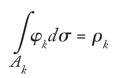
where φ(.) is the usual standard bivariate normal density with parameter ρ and σ(.) is the Lebesgue measure.
The other issue regards something that always undermines correlation: It doesn’t imply causation. We may observe a high positive correlation between the number of ice creams sold on a beach and the number of shark attacks, but that connection is spurious: It’s not quite right to say that ice cream causes shark attacks. Lurking variables like the number of people on the beach may affect both variables similarly. With the bridge-formation tool established (polychoric correlations for us), this can be fixed by creating the network the right way, through a Markov Random Field, exemplified by Figure 1. The edge dependencies are conditional. When two attitudes are dependent—positively or negatively—they are truly so after controlling for (or removing the effects of) all other variables. It was not a spurious or a non-sense relationship. Note that these other variables being controlled for include all those the survey collected information about, except, of course, the two under investigation. Though this is a pretty thorough list of 128 details, there may be other factors beyond these that could affect opinion.
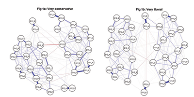
Figure 1. Markov random fields formed through polychoric correlations for those who identified as very conservative (1a, left panel) and very liberal (1b, right panel). Notice, in both cases, the separation between the 11 and the 12 crowd.
Formally, Markov random fields are undirected networks (showing connections among tendencies, taken as nodes) whose edges can be thought of as showing the extent of conditional dependencies between two nodes (assuming the other nodes don’t interfere with this relationship). The edge weights are often taken to be partial (or polychoric) correlation type quantities, and these random field models are implemented—the edge weights are estimated through Lasso-type regularization techniques (where a large value of the regularizer or the “penalty parameter” may lead to wrongly missing true edges, while a low value may wrongly bring in false edges; the optimal value is chosen through minimizing the BIC criteria).
A Tale of Two Networks
It may be quick to construct one MRF network out of all survey participants and talk in generalities, highlighting which attitudes are conditionally entangled with which. When we look at portions of the sample, however, nuances emerge, and subtler questions are formed. Network 1A in Figure 1, for instance, was formed out of participants who identified themselves, politically, as very conservative; 1B out of those that were very liberal. On the conservative network, questions 11 and 12 on the same sub-theme, Q, shared a strongly negative bond. Question 11 summarized what ought to be and 12, what is. Conservatives who feel it is extremely important to avoid major pay gaps between CEOs and average employees feel, generally, companies are doing “poorly” reducing that gulf. The solid red bridge between these two brings out the mismatch between what should have been and what is—the disjunct between the dream and the evidence. The corresponding connection on the liberal side is almost nonexistent, suggesting a sort of conditional independence. How do you test whether this disagreement is substantial enough to not have been caused by random chance or check whether the total amount of blue and red connections match across the two networks? In short, how do you test the statistical equality of the two networks? We may have seen similar comparisons through tests for two independent samples made of independent copies of random variables: boys’ and girls’ IQ scores, for instance. How do you extend these to networks, which are fundamentally a description of dependencies?
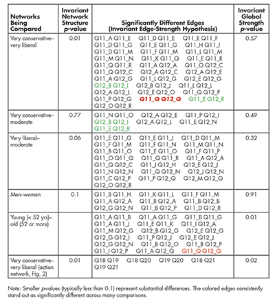
Permutation tests hold the key. They begin by recording an appropriate statistic—the absolute difference in this case between the 11Q–12Q edge weights from the conservative and liberal sides. The conditional edge dependency described in the previous section between these two nodes was estimated (through lasso regression—in case you’re curious—that does variable selection, ensuring true edges are not missed, and false edges are not considered) to be −0.15421 on the conservative side (notice the heavy red color in Figure 1) and −0.001684 on the liberal side (notice the fainter red). The absolute difference between the edge weights becomes |−0.15421 – (−0.001684)| = 0.1525. This 0.1525 becomes the observed value of the test statistic for us. Next, we need some reference against which to judge whether this value is too large, some benchmark that shows typical values of this difference in case the political labels did not matter, or are under the “null” assumption. This null distribution is made by randomly assigning people to parties and measuring the 11Q–12Q edge weight differences. Only 4.57 percent of those values exceeded the observed statistic, which makes 0.1525 unlikely to be a chance difference (please see Table 2). Conservatives and liberals genuinely seem to disagree on how automatic the 11Q–12Q connection needs to be. What we checked is known as the hypothesis for invariant edge strength. Formally, the null hypothesis here is
![]()
where wCij and wLij are the (true) edge-strengths joining nodes i and j on the conservative and liberal sides, and the test statistic used here was E (wCij , wLij) = |wCij – wLij|. Other hypotheses may be formed and tested too. Since a network is fundamentally a collection of edges, all of them, in some way or another, deal with edges—one at a time, or many. For instance, the hypothesis of invariant network structure is stricter, claiming all the edge strengths are statistically equal across the networks. The test statistic changes naturally, and we look at the maximum of the edge-weight differences and reject the null assumption in case this maximum is intolerably big. A great strategy is to first check the hypothesis of invariant network structure, in case it is rejected (indicating at least one edge strength varies across the networks), then move on to test the hypothesis of invariant edge strength to work out which edges are substantially different, much akin to the global F-test and the separate t-tests, to borrow a regression analogy.
Another kind of test lifts our focus from a narrow, local power-edge analysis to a larger collective plane and checks whether the overall connectivity has remained more or less similar across the two networks. This is called the hypothesis of invariant global strength. Using similar notations and assuming there are p nodes, the null assumption here may be framed as
![]()
with the test statistic being ![]() and the p-values found through measuring the proportion of times—as discussed before through the other tests—that the “null” values exceed the observed value of the statistic. These results are recorded in the last column of Table 2.
and the p-values found through measuring the proportion of times—as discussed before through the other tests—that the “null” values exceed the observed value of the statistic. These results are recorded in the last column of Table 2.
Politics was an example. Other factors may divide participants too: gender; age; wealth; etc. Table 2 records some of these comparisons. However, none of these cases’ differences were as stark as the one in the very conservative—very liberal comparison, both in terms of the overall (global) network structure (the tiniest p-value: 0.01) and the number of significantly different edges detected. Some edges stay consistently different across these populations. While conservatives give the impression that the conditional dependence between the importance of “promoting diversity, equity, and inclusion” and whether businesses are “making money in ways that are ethical” is quite strong, liberals disagree (the 11E–12 R connection). While liberals show the importance of reducing wage gaps is strongly automatic with how businesses are doing making the world a better place, conservatives disagree (the 11Q–12C connection). Despite these differences, there are many edges (more, in fact) on which the two sides agree. Whether we let businesses get away with dodgy ethics and loose morals, therefore, depends, in part, on the section of the population we are interviewing.
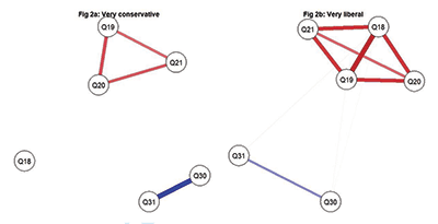
The survey questions seen so far deal with people’s opinions: whether they feel an issue matters; whether businesses, in their opinion, are doing enough in that regard; etc. The binary questions 18, 19, 20, 21, 30, and 31 are different (please see Table 1). They are action questions. They put the respondents in a spot, checking whether they will act if prompted: paying extra to a business that does good for the public or embracing a pay cut if that means joining such an organization, etc. These action responses are binary, and the edges are not made through polychoric correlations anymore (partial correlations of zero do not show conditional independence here), but they still represent associations among mindsets: They are the coefficients when one attitude is logistically regressed on the others. Differences exist between conservatives and liberals on these action items also (please see Figure 2 and Table 2).
From edges, we may turn our attention to nodes as well. Which ones control the hub of activity? The ones with the most correlation attached. For conservatives, it is 12M (whether the business functions in a way that is sustainable for the environment); for liberals, it is 11F (whether the business offers fair wages to workers of all types). Those are the vertices most entangled with the rest—the nuclei around which the networks revolve—and poking them will create the maximum disturbance, the biggest ripple throughout the network.
While the questions we have focused on (those shown in Tables 1 and 2) are not randomly chosen out of the larger “population” of 128 questions, they are, in a way, some key ones, touching on vital issues such as politics, age, and gender, where divisions in society are generally thought about. Viewed this way, there were certain details like the time a respondent took that may be temporarily ignored as non-key (they are not correlated with the key ones, either). Based on these preliminary findings, a fuller analysis can be launched with other key questions like, “How much are you willing to pay for a t-shirt,” which could be a proxy for their wealth.
There was a time when hearing someone’s ambition of becoming a successful businessperson evoked a specific image—the stereotypical one of someone’s steadfast toil to maximize profit at any cost, to the exclusion of everything else—and “ethical business” sounded like an oxymoron. Things have changed. The ways those profits are accrued have begun to matter. A typical consumer is realizing the ills that ail these companies and would not turn a blind eye to those that abandon workers’ welfare or environmental concerns. Firm statistical analysis will help us understand whether senseless profiteering has given way to saner compromises, where people’s attitudes toward certain practices vary according to their position on the political or economic spectrum. Large and reliable data—such as the ones collected by the Gallup team—make the testing of these hypotheses possible.
Developed originally to shed light on individuals that are naturally interconnected—friends on Facebook, for instance—network science soon stirred interests beyond its immediate circulation. Whatever the survey, differences in people’s backgrounds are unavoidable. They are in different stages of their career, they have different demographic features, or they sit on different sides of the political aisle. Whether what divides them also changes the degree to which one attitude depends on another is, however, far from trivial. An MRF formed through polychoric correlation brings the intricacies to the fore, connecting perspectives instead of people, showing the complexity of their relationship—whether conflicted or symbiotic—and the chief channels of communication dependence flow, the key islands around which that flow eddies.
Further Reading
Epskamp, S., Cramer, A.O., Waldorp, L.J., Schmittmann, V.D., Borsboom, D. 2012. qgraph: Network visualizations of relationships in psychometric data. Journal of Statistical Software, 48(4):1–18.
van Borkulo, C.D., van Bork, R., Boschloo, L., Kossakowski, J.J., Tio, P., Schoevers, R.A., Borsboom, D., Waldorp, L.J. 2022. Comparing network structures on three aspects: A permutation test. Psychological Methods, 28(6):1273–1285.
About the Author
Moinak Bhaduri is an assistant professor of mathematical sciences at Bentley University. Rooted in applied probability, Bhaduri studies spatio-temporal Poisson processes and others that are natural generalizations like the self-exciting Hawkes or log-Gaussian Cox processes. His primary interest includes developing change-detection algorithms in systems modeled by these stochastic processes, especially through trend permutations. His research had found applications in computer science, finance, reliability and repairable systems, geoscience, and oceanography. This work was supported, in part, by the Research Enhancement Grant from the American Mathematical Society and the Simons Foundation. The author also gratefully acknowledges Bentley University’s summer research support.

