
A Curveball Index: Quantification of Breaking Balls for Pitchers
Miles per hour has been the rating system that pitchers all over the world are held to for their fastball. Having a standardized scale makes it easy to compare, value, and track progress of different pitchers everywhere. Having a metric that applies to everyone allows us to easily compare pitchers and recognize talent. Thus, the rating system for the fastball has become the worldwide standard. However, there is no similar standard for rating breaking balls, of which the curveball is one type. A curveball is a pitch that begins straight, like a fastball, and then suddenly moves vertically downwards due to spin placed on the ball. The curveball’s effectiveness is mainly in the difference of movement, and unexpected change from a fastball, which is a more frequently occurring pitch. The purpose of this paper is to develop an index for quantifying the quality of curveballs and to suggest how this index may be used to improve pitcher training and scouting.
The idea was to observe a variety of curveballs—good and bad—measure their key components, and generate an index from them. It originated with the class project of a student (Jarvis Greiner) in my (Jason Wilson) statistics class. Jarvis was a pitcher on our baseball team and a film major.
We used a video production studio with three pitchers from our baseball team to collect our own data. We measured the rise, breaking point, knee distance, and total break of each pitch, along with a quality rating by a pitching coach.
Jarvis’ initial idea for the index was to assign points to the breaking point(+), total break(+), rise(-), and knee distance(-) and sum the terms using the sign indicated. The breaking point and total break were added because the bigger they are, the better the curveball. Conversely, the rise and knee distance were subtracted because the bigger they are, the worse the curveball is.
This intuitive formula actually worked surprisingly well. However, using multiple regression, we were able to generate the optimal index from the four variables (good model fit, R =0.73, p-value = 2.2 x 10⁻¹⁶). The model details and the comparison between the intuitive model and the regression model can be found in the Analysis section. The resultant index appears promising and, given data for a pitcher, could be used by coaches and pitchers to track progress and adjust technique. It also could be used by scouts as a talent metric other than the fastball.
Data
To pull off our task, we needed data. During the fall 2009 semester, the Biola production studio was arranged with three cameras and reference markers in the background (see Supplemental Material for technical set-up information). Three pitchers from our National Association of Intercollegiate Athletics (NAIA) baseball team threw 10 curveballs each, individually recorded by the cameras (Figures 1 and 3). After each pitch, the coach rated its overall quality on a scale of 0 to 100. This quality rating is the response (dependent) variable. Later, the footage was analyzed to determine the values of five numeric variables used to characterize the path of each pitch.
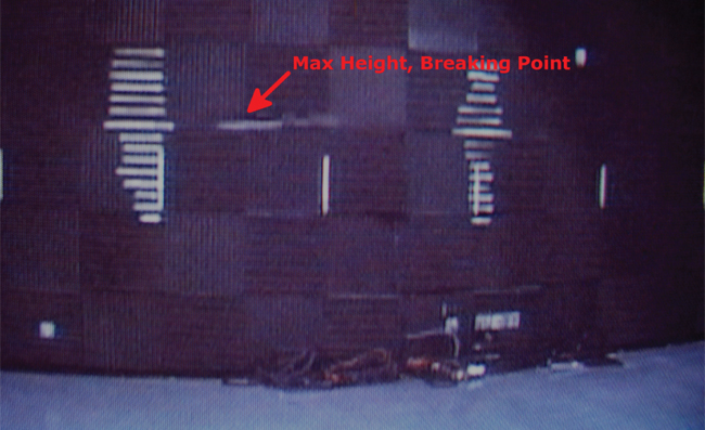
Figure 1. Still photo from Camera 2 showing how the maximum height and breaking point of a pitch was obtained
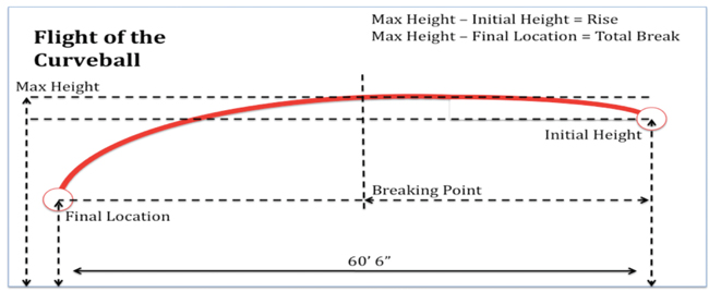
Figure 2. Diagram of the flight of the curveball. The four variables collected (Rise, Breaking Point, Knee Distance, and Total Break) are calculated from the variables measured from the video footage, shown on the diagram.
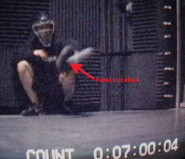
Figure 3. Still photo from Camera 3 showing how the final location was obtained
One of the main questions people ask when hearing about our study is, “Why didn’t you use a batter, instead of a pitching coach, to really see how good the pitches were?” There are two main ways to go about this kind of study: (1) using a batter during game play and (2) using a pitching coach in a controlled experiment. To understand our rationale, let us contrast these approaches. The first is observational, the second is experimental. The first could use major league baseball stadium PITCHf/x data, the second requires experimental data collection. The first would require a pitch-type classification algorithm, the second does not. The first requires a binary response (hit/miss) regression model, the second allows a conventional numeric response. Our purpose was to develop an easy-to-use index for use by all pitching stakeholders.
The experimental design approach is preferable for model development, the process has less variation, the model interpretation is simpler, the method can be employed by any baseball coach (not just major league with PITCHf/x), and the study is reproducible. We agree that the first approach could make a good and interesting study, but we chose the second because it suits our purposes better.
For each pitch, data were collected on the following five variables: Initial Height, Max Height, Breaking Point, Final Location, and Knee Distance. The five measured variables were converted into four explanatory (independent) variables: Rise, Breaking Point, Total Break, and Knee Distance. The pitch speeds were all consistent with the speeds of good curveball pitches. The measured variables are defined as follows (Figure 2):
- Initial Height: vertical height of the ball as it leaves the pitcher’s hand (in.)
- Max Height: maximum vertical height the ball achieves (in.)
- Breaking Point: horizontal distance the ball travels from the pitcher until it begins to break (curve downward) (ft.)
- Final Location: vertical height of the ball as it stops (in the catcher’s mitt) (in.)
- Knee Distance: |Final Location – 18| (in.)
The measured variables were converted to the following four independent variables:
- Rise: Max Height – Initial Height
- Knee Distance: as measured
- Total Break: Max Height – Final Location
- Breaking Point: as measured
To summarize, the first three variables are vertical and the last one is horizontal. The rationale for including each variable is as follows:
- Rise: The less rise, the harder it is for the hitter to tell it is a curveball. None of the other pitches rise, so if the batter notices a rise in the ball, they can anticipate the curve.
- Knee Distance: The 18-inch benchmark has been selected as the ideal vertical ball stopping height for three reasons. First, it is in the strike zone (in particular, at the bottom of the strike zone). Second, the closer the ball is to the knees, the better for luring the batter. Third, it is more difficult to hit the ball when it is lower.
- Total Break: More break means more hitter head and eye movement, making it harder for the batter to judge where the ball will wind up.
- Breaking Point: The longer the breaking point (closer to the batter before the ball breaks downward), the less time the hitter has to react.
A few sample data points are shown in Table 1. The full data set may be found in the supplementary material.
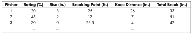
Table 1—Sample Data Points from the Four Variables Collected from Three Pitchers
Analysis
A multiple regression model was fit to the data (see Multiple Regression.pdf). All statistical work was done using R (www.r-project.org; see Curveball Index Supplemental Material for the R scripts). After experimenting with different models (intercept/no intercept model, quadratic terms, interaction terms, and a pitcher effect), the following model was found to be the best:
rating = 2.51rise + 1.88breakpoint – 0.47knee_dist + 0.51total break (1)
The model quality is good. The probability that the model coefficients would be what they are, or farther away from zero, due to mere chance is less than 2.2 x 10⁻¹⁶. The proportion of the variation in the Rating unexplained by the no intercept model is the error in the residuals (1786) divided by the total Rating error (6527), or 1786/6527 = 0.27, which is 27%. In other words, the model is able to account for R2* = 73% of the variation in the Rating on the basis of Rise, Breakpoint, Knee Distance, and Total Break.
You may be thinking, “OK, now what does this model mean?” The key to the meaning lies in interpreting the model coefficients. The model coefficients can be interpreted in two ways. The first is in absolute terms, according to the original Rating scale. The second is in relative terms, according to their relative effect on the predicted Rating.
Throughout the discussion, please keep the following in mind. The response variable, Rating, is on a scale from 0 to 100 for the quality of the curveball thrown. In the data, Rating was measured from a low of 18 to a high of 75, giving a range of 75 – 18 = 57. The model is only valid for predicting Rating within the range of the data, 18 to 75. Going beyond this range would be extrapolation, which is not justified by regression models.
The model coefficients may be interpreted in absolute terms as follows. For a given response variable, holding the other three constant, each coefficient may be interpreted as the number of points the Rating would move if the variable moved one point. For example, if Breaking Point, Knee Distance, and Total Break were held constant and the pitch were raised (+) one inch, then, on average, Rating would go down (-) 2.51 points. If the same pitch were lowered (-) one inch, then, on average, the Rating would go up ( – – = +) 2.51 points. As a second example, if the Rise, Breaking Point, and Knee Distance were held constant and the Total Break were increased by one foot, then the Rating would increase 0.51 points on average. If the Total Break were decreased by one foot, then the Rating would decrease 0.51 points on average.
Further information regarding the precision of the coefficients may be found in the second column of Table 2. A 95% confidence interval (CI) is given for each coefficient. A 95% CI means that if God were to drop a golden scroll from heaven with the ‘true’ model of the curveball rating for all NAIA pitchers (or whatever population our pitchers come from), then there is a 95% chance that each of our CIs would contain the ‘true’ model coefficient. For example, for Rise, we are 95% confident that the true coefficient lowers Rating by 3.8 to 1.2 points per inch the curveball rises on average.
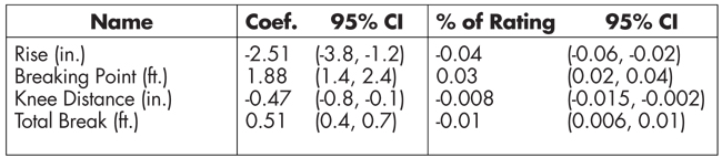
Table 2—Model Coefficient Data
The second column contains the model co-efficient, followed by the 95% confidence interval in parentheses. The third column contains the % of Rating a change of one unit would produce, on average, from this data.
The model coefficients may be interpreted in relative terms as follows. The third column of Table 2 refers to the relative amount of change in Rating due to change in the variable. It is obtained by dividing the coefficient (95% CI) by the range of the observed data, which is 57. For example, if Breaking Point, Knee Distance, and Total Break were held constant and the pitch was raised one inch, then, on average, the Rating would go down by 0.04 (-0.06; 0.02), or 4% (-6%; -2%). These % changes are comparable to what is obtained when using a model with the log of the response variable.
We collected data using three pitchers. When we built the model using Pitcher as a factor, the Pitcher effects were not significant (p-value = 0.41; 0.69; 0.58), indicating the pitchers were similar in skill and did not contribute a significant source of variability. If this concept were adopted by a coach or scout and sufficient data were collected, then computing the pitcher effect could be used to compare different pitchers.
In summary, the model coefficients show how much effect each component has on the curveball Rating, and in what direction. This information could be used by scouts and sabermetricians to compare pitchers. It also could be used by pitchers and their coaches, for example, to identify which adjustments to their curveball would likely yield the most improvement. Keep in mind that, although Rise apparently has the largest effect since its coefficient is the largest, this is simply due to the units of measurement. For example, if Rise were measured in 1/8-inch increments, its coefficient would be -2.51/8 = -0.31, while the others would remain the same, making it appear as the smallest effect. Since significant interactions and higher ordered terms were not found, the one who attempts to conceptualize the model can reasonably conceive of all four explanatory variables independently summing to the final Rating.
There is one other consideration for a multiple regression model to be valid. It turns out that, even though a regression model may be a good fit to the data and satisfy the assumptions, if the explanatory variables exhibited significant linear dependencies (i.e., multicollinear), then the model would be unstable. If the model were unstable, then slight changes in the data would significantly alter the coefficients, changing their interpretation.
In our case, the very appeal of the model is dependent upon the understanding of the coefficients. Fortunately, the regression variables are sufficiently linearly independent. One way to see this is through viewing the correlation matrix in Table 3, where every entry shows the correlation coefficient between two variables. The correlation matrix shows that no two variables are strongly correlated (|correlation| < 0.80), and there is a mixture of positive and negative correlations. The explanatory variables certainly have some dependence, but not enough to be a problem. (There are several technical ways to check for multicollinearity. One is if the condition number of the data matrix is over 1,000. For our data, the condition number is 24.1. A second technical check is if one or more of the variance inflation factors is over 10. The variance inflation factors are 9.4, 5.6, 4.2, and 3.8. Both techniques indicate multicollinearity should not be a problem.)
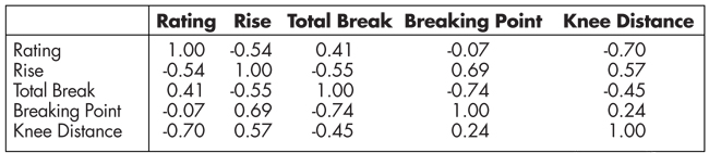
Table 3—Correlation Matrix for the Pitching Data
The correlation between all regressor variables is weak to moderate, and the direction of each correlation with ‘rating’ is as predicted.
I (Jason) would like to conclude this section with a pedagogical remark. In the introduction, we mentioned Jarvis’ intuitive model. Using the notation above, that model may be written as the following:
index = 40rise + 20breakpoint – 20knee_dist + 20total break (2)
Clearly, this intuitive index is on a different scale than the % rating given by the pitching coach. However, the correlation between this index and the actual rating is r = 0.74, which means 100 (0.74)2% = 55% of the variation in the rating is explained by the data. While this is below the amount found by the regression model (73%), the signs on the coefficients are all correct and the magnitude of the coefficients is roughly comparable. I find this insight impressive (we did not cover multiple regression in the class). On this basis, I urge the readers who are educators to provide similar opportunities to your students. This could enable them to use their own expertise to make personal discoveries leading to not only great satisfaction, but also an unforgettable and hopefully contagious statistical education!
Conclusion
The goal of the curveball index described has been to quantify the value of a curveball and propose a standardized rating system, or metric, for it. This would not only allow a pitcher’s progress to be tracked and provide a training tool, but it would facilitate comparison between all curveballs and curveball pitchers. Not only pitchers and coaches, but also scouts, baseball fans, and sabermetricians would benefit from such a rating system. The proposed linear model shows that the intuitive relationship between rise (lowers curveball quality), breaking point (the longer the better), knee distance (the closer to the bottom of the strike zone the better), and total break (the bigger the better) is best. That is, there are no interactions or quadratic relationships. This supports not only the plausibility of the model, but also its portability.
With respect to the specific regression coefficients given in our model, they are preliminary and subject to revision after further data collection. This is indicated by the confidence intervals for the coefficients in Table 2, which would narrow with further data. The contribution we intend to make is the use of the four variables, as defined, in the regression model to form a standardized curveball rating system.
It is noted that other height variables in place of rise + total break could be used equivalently in the model (in particular, final height + total break or initial height + rise). However, we prefer rise + total break because they remove the artifact of pitcher height and are the variables pitchers and coaches really think about. If our concept were adopted, the coefficients would need to be updated with more data from different pitchers with different skill levels rated by different coaches. We predict the coefficients would change, but the signs and relative relationship between coefficients would remain the same. After such refinement, the coefficients should probably be rounded to obtain a “nice” formula for wider adoption by the baseball community. It is conceivable that a standardized model could be adopted, while individual pitching coaches might develop proprietary models for “in-house” use.
Last, our work could be expanded in the following ways. The Knee Distance variable might be adjusted, possibly weighting distances below the knee twice as much as above. Using a speed gun, we could add Speed as an additional variable and hopefully increase our 73% model variation explained.
For even further development, we are considering generalizing the model to other breaking balls, such as the “slider.” Such work would provide data useful not only for rating pitching quality, but also classification. If enough data were available, a pitcher effect could be computed and used to compare different pitchers. If the coefficients of our current model were updated and adopted, with a suitable classification algorithm, then PITCHf/x curveballs could be assigned our curveball index scores, thereby realizing the goal of major league baseball pitch/pitcher standardized curveball comparison.
Further Reading
Alan, Nathan. 2010. MLB PITCHf/x Data. (4/10/12).
Albert, James. 2006. Pitching statistics, talent and luck, and the best strikeout seasons of all-time. Journal of Quantitative Analysis in Sports 2(1). DOI: 10.2202/1559-0410.1014.
Albert, James. 2009. Exploring PITCHf/x Data. Keynote address, The Institute of Mathematics and Its Applications 2nd International Conference on Mathematics in Sport.
Fast, Mike. 2008. How will ball tracking analysis change the game? The Hardball Times. (4/10/12).
About the Authors
Jarvis Greiner—from Edmonton, Alberta, Canada—earned his BA in cinema and media arts production as a multi-sport, dean’s list student athlete at Biola University in La Mirada, California. As a former varsity baseball player, Greiner has three passions: baseball, statistics, and video production. This makes him excited about making curveball quantification practical to the baseball community. His goal is to make this index a standard, much like mph is to judging velocity.
Jason Wilson earned his PhD from the University of California, Riverside, and is an associate professor of mathematics and statistics at Biola University. Wilson’s research specialization is in the application of statistical methods to biotechnology. When not too busy teaching, he enjoys statistical consulting. Most recently, he has been doing undergraduate student-collaborative research in such areas as Yahtzee calculations, crime data, and the integration of statistics with the Christian faith.


