Steven Tijms

Seeing Is Believing

Throughout the history of mathematics, quite a few mathematical problems have achieved celebrity status outside the circle of mathematicians. Famous problems such as squaring the circle or proving Fermat’s last theorem have intrigued thousands of people over the centuries. But almost no mathematical problem has been as fiercely and widely debated as the Monty Hall problem—not because the problem defies a solution, but because its solution runs completely counter to what we intuitively expect.

The Monty Hall problem, also known as the Three Doors problem, was first posed and solved by biostatistician Steve Selvin as early as 1975, in a letter to the editor in The American Statistician. Inspired by the then-hugely popular TV game show “Let’s Make a Deal,” Selvin named the problem after its legendary host, Monty Hall. Several of Selvin’s colleagues disputed the solution he provided, so he submitted a second letter to the editor, including a formal proof, and there it ended. That is, until September 9, 1990, when Marilyn vos Savant, in her weekly “Ask Marilyn” column in Parade magazine, answered a reader’s question about a game show very similar to “Let’s Make a Deal”:

“Dear Marilyn: Suppose you’re on a game show, and you’re given the choice of three doors. Behind one door is a car, the others, goats. You pick a door, say number 1, and the host, who knows what’s behind the doors, opens another door, say number 3, which has a goat. He says to you, ‘Do you want to pick door number two?’ Is it to your advantage to switch your choice of doors?” –Craig F. Whitaker.

At first glance, the solution seems pretty straightforward. With two doors left, one of which has the car behind it and the other a goat, chances must be 50-50. In other words, it should make no difference at all whether you switch doors or stick to the door of your initial choice. But vos Savant replied: “Dear Craig: Yes, you should switch. The first door has a 1/3 chance of winning, but the second door has a 2/3 chance.”

Unlike The American Statistician with its select readership of specialists, Parade magazine is read by millions of people across the United States. vos Savant’s reply provoked a nationwide debate. On July 21, 1991, the New York Times even ran a front-page article about the heated controversy. The article was picked up by foreign newspapers and soon the Monty Hall problem also conquered Europe and the rest of the world.

vos Savant herself was flooded by a surge of disbelief. She received more than 10,000 letters from readers of her column, the vast majority of whom were absolutely convinced that she was wrong. Among them were many PhDs and a strikingly large number of mathematicians. One understanding mathematician kindly offered vos Savant some comforting words: “You made a mistake, but look at the positive side. If all those PhDs were wrong, the country would be in some very serious trouble.”

In a second column about the problem, vos Savant used a table of six possible outcomes to prove she was right. The reactions she then received were only more vicious and sarcastic. One reader, for instance, wrote: “…I am sure you will receive many letters on this topic from high school and college students. Perhaps you should keep a few addresses for help with future columns.” In other words, vos Savant, although once listed in the Guinness Book of Records for her exceptionally high IQ, supposedly did not have the slightest understanding of probability.

Then, in a third column on the problem, vos Savant changed strategy. She called on math classes across the United States to take a die, three paper cups, and a penny; turn the cups over; and hide a penny under one of the cups. Then the students—one being the ignorant contestant, another the knowing host—should simulate the game, repeating each of the two strategies, switching and sticking, 200 times.

As many as 50,000 students answered her call. A student wrote: “At first I thought you were crazy, but then my computer teacher encouraged us to write a program, which was quite a challenge. I thought it was impossible, but you were right!” And another one: “I also thought you were wrong, so I did your experiment, and you were exactly correct. (I used three cups to represent the three doors, but instead of a penny, I chose an aspirin tablet because I thought I might need to take it after my experiment.)” Almost all experiments confirmed that switching doors doubles the chance of winning.

vos Savant was right after all. The massive experimental confirmation marked a turning point. Many people were now letting her know that they had changed their minds. A substantial minority, however, persisted in their mistaken opinion. A scientist wrote, “I still think you’re wrong. There is such a thing as female logic.”

Over the years, many ways to solve the problem have been proposed, from simple word proofs to Bayesian demonstrations. An easy way to visualize that switching doors doubles your chance of winning is this thought experiment. Imagine that you could repeat picking a door 15,000 times. Then, on average, you would pick the winning door about 5,000 times (one-third of the time) and a losing door about 10,000 times (two-thirds of the time). If you are given the option to switch doors, you had better switch.

Today the question is no longer whether vos Savant was right, but why so many people were mistaken, and what’s more, why they were so deeply convinced that she was wrong and they themselves were right. Especially since many of them were capable mathematicians. The outrage was considerable: In their minds, vos Savant was only contributing to statistical illiteracy in the nation. Some even suggested that she would do well to quit writing for Parade magazine, either voluntarily or involuntarily. How could even trained mathematicians be so wrong?

Some mathematicians claimed that the problem was not well defined, but to the vast majority of readers of vos Savant’s column, most of whom were well-acquainted with Monty Hall’s game show, the rules were crystal clear. The car was placed behind one of three closed doors and only the host knew which door. After the contestants picked a door, the host opened one of the other two doors, but, of course, never the door with the car behind it. The contestants, who were aware of this, were then offered a final choice: Stick with the door of their initial choice or switch doors.

In the 1991 front-page article in the New York Times, probability expert Persi Diaconis confessed to columnist and reporter John Tierney that he could not remember what his first reaction had been, because he had known about the problem for so many years, but that with similar problems, his first reaction had been wrong time after time. “Our brains,” he commented, “are just not wired to do probability problems very well.”

Could the answer be found in the way our brains function?

The Power of Illusion

In recent years, the Monty Hall problem has become the subject of extensive psychological research and has been hailed as a model example of a cognitive illusion. Cognitive illusions occur when our judgment is misled, just like optical illusions occur when our eyes are tricked. According to mainstream cognitive psychology, cognitive biases and illusions originate from the application of intuitive heuristics—a kind of built-in mental shortcut used by our intuition to quickly reach a judgment in situations of uncertainty. If that is so, what intuitive heuristic could underlie “the Monty Hall illusion”?

Many psychologists approach the Monty Hall problem not as a probability problem but as a purely cognitive dilemma: whether to switch doors or stick with your initial choice. They thereby take the sting out of the problem. In 2014, social psychologist Donald Granberg published a monograph about the dilemma, entitled The Monty Hall Dilemma. A Cognitive Illusion Par Excellence, in which he examined several possible psychological heuristics that could play a role in the dilemma.

Psychological research shows that most subjects decide to stick with their initial choice and that several psychological factors play a role in this decision. One of these factors is counterfactual or “what if” thinking. In Granberg’s own words, “People avoid switching in the Monty Hall Dilemma, in part, because they anticipate they would feel worse if they switched and lost than if they decided to stick and then lost.” Another psychological factor is the illusion of control. As Granberg wrote, “When people make the initial selection, this very act of choosing may create an illusion of control in their minds that causes them to be reluctant to abandon that choice.”

These two irrational heuristics appear to be the most common. But as real as these psychological factors may be, are they really key to most subjects’ decision to stick with their initial choice?

The psychological research was set up as word-problem experiments modeled after Monty Hall’s game show. But why not consider Monty Hall’s own television show as a psychological experiment? An experiment in a real-life setting, conducted by Hall himself—after all, he both produced the show and hosted it for nearly three decades.

In the New York Times article, Tierney quoted Hall as not being surprised that even experts insist that the probability is 1 in 2 because it’s the same assumption contestants would make after he showed them there was nothing behind one door. “They’d think the odds on their door had now gone up to 1 in 2, so they hated to give up the door no matter how much money I offered.”

According to Hall, the number one reason why contestants decided to stick with their initial choice was simply their belief that their chances of winning had increased from 1 in 3 to 1 in 2. Clearly, this observation makes sense. If the contestants hadn’t believed it, then sticking with their initial choice would not have been a wise thing to do. They would probably all have switched doors. In other words, counterfactual thinking and the illusion of control may well have played a role in the contestants’ decision to stick with their choice—but only as secondary factors. At the root of their decision lies the stochastic misconception that we set out to explain.

It looks like we are back where we started, but that is not entirely true. The psychological detour has suggested a way for us to move on. Just as cognitive psychologists treat the decision of most subjects to stick with their initial choice as a cognitive illusion, we might treat the belief that the probability of winning increases to 1 in 2 as a mathematical illusion; that is, an illusion based on some intuitive stochastic heuristic. That would explain why so many people were mistaken and why the solution to the Monty Hall problem feels so counter-intuitive. Even the Hungarian mathematical genius Paul Erdős initially thought vos Savant’s solution was impossible.

A year before his death in 1996, Erdős heard about the Monty Hall problem from his colleague and compatriot Andrew Vazsonyi. Erdős couldn’t belief that switching doors would make a difference. A decision tree did not convince him. He asked Vazsonyi to give him a reason why switching doors mattered. Vazsonyi couldn’t find one, so he had the computer simulate the show game 100,000 times. This time, Erdős was convinced, but he insisted that he still did not understand the reason why.

Many people will share Erdős’s feeling of discontent: “Okay, Marilyn is right and I’m wrong, but why?” Computer simulation will not give you the answer, nor will a Bayesian proof provide you with an “Aha!” experience. How can something that is wrong seem so convincingly right? Or more specifically, what makes the solution to the Monty Hall problem so counterintuitive?

The late Ruma Falk, an expert in the psychology of probability, asked the same question in her article “A Closer Look at the Probabilities of the Notorious Three Prisoners,” which she wrote in 1991 when the controversy over the Monty Hall problem was at its peak.

The Uniformity Belief

The Three Prisoners problem—a classic brain teaser introduced by Martin Gardner in his “Mathematical Games” column in Scientific American in 1959—bears a strong resemblance to the Monty Hall problem. Its solution is also completely counter-intuitive. It contradicts the same strong stochastic intuition that, according to Falk, was responsible for the surge of disbelief that flooded vos Savant.

Falk observed that “Marilyn’s attackers all believe in the equiprobability of the two remaining possibilities” and that they are not only numerous but also highly confident, “as if there is intrinsic certainty to that belief.” She also noted that this belief is “second nature for many naïve, as well as statistically educated solvers.” She named it the uniformity belief. It says that if only two alternative possibilities remain, they are equally probable.

Falk’s observations precisely capture the thinking of many of vos Savant’s critics. With two doors left, one with a car behind it and the other with a goat behind it, intuition tells us that the chances must be 50-50. No further mathematical underpinning seems necessary: It’s self-evident. This also explains why so many of those critics directed their criticism at vos Savant herself rather than at her solution. vos Savant defied common sense; she must be out of her mind!

But her critics were wrong themselves. In truth, switching doors will double your chances, so apparently, two remaining alternative possibilities need not be equally likely at all. But if that’s the case, then why is the uniformity belief such a compelling and self-evident intuition? How can it lead so many people astray?

In a later article entitled “The Allure of Equality: Uniformity in Probabilistic and Statistical Judgment,” Falk set out to find the source of the uniformity belief, but in the end, concluded that the roots of the uniformity belief are still not fully understood. In the same article, however, she also suggested that the belief might be explained as “a quest for fairness and symmetry.” Without realizing it, she held the keys in her hands.

The Mundane Roots of Equipossibility

vos Savant was criticized for not having the slightest understanding of elementary probability. Did that mean the uniformity belief could somehow be embedded in our elementary knowledge of probability? Almost every elementary textbook says that the probability of an event is the ratio of the number of favorable possible outcomes to the total number of possible outcomes. If there are only two possible outcomes, one favorable (the car), one unfavorable (a goat), then the probability is clearly 1/2.

And yet this textbook definition cannot be the source of our uniformity belief, simply because, as Falk observed, the same belief is also second nature for many statistically naïve solvers. That doesn’t say, however, that the two are not related at all. The textbook definition assumes that the various outcomes are all equally possible. The uniformity belief is, so to speak, built in. Finding the origin of this mathematical assumption of equipossibility may also shed light on the roots of our intuitive uniformity belief.

The standard formulation of the textbook definition of probability, as is commonly known, stems from the French mathematician and polymath Pierre-Simon Laplace (1749–1827). It is known as the classical definition of probability. In his “Philosophical Essay on Probabilities,” a non-technical résumé of his mathematical work on probability, Laplace calls the definition the first principle of probability. Its assumption that the various possible outcomes are all equally possible is the second principle. Without this assumption, the definition would make no sense. But where does this assumption come from?

Laplace’s essay ends with a brief historical survey of probability calculus, concluding with the memorable words: “It’s remarkable that a science that began by considering games of chance should itself be raised to the rank of the most important subjects of human knowledge.” That is, it all began with the mathematical study of games of chance. In the early days, these were mostly dice games.

Playing dice is practically as old as human history. Initially, people used the four-sided knuckle bones of goats and sheep, called astragali, but the six-sided die as we know it today also goes way back. It was invented at least 5,000 years ago. In ancient times, betting on the outcomes of two or three dice was widespread, and in Europe, it was a popular pastime well into the 17th century.

These dice games lie at the historical roots of probability calculus. Long before, Laplace writes, players already knew the ratios of favorable to unfavorable possible outcomes in the simplest games. Bets were settled by these ratios. Today, we call these ratios the odds. The odds tell you how much closer you are to winning than to losing.

In the 16th century, a general betting rule was first formulated by the colorful but almost forgotten Italian mathematician Girolamo Cardano (1501–1576). Cardano, himself an avid gambler, wrote in his short handbook on gambling De ludo aleae (On Games of Chance) that fairness is the fundamental principle of all gambling. But how do you know if a game is fair?

Cardano’s rule states that a game is fair if the ratio of bets is proportional to the ratio of favorable to unfavorable outcomes. Then, both players have equal expectations of profit and loss. If, for example, the odds are 1 to 4 against you, then you should bet a amount of money that is four times smaller than the amount of your opponent’s bet.

This obviously only makes sense if the various outcomes in these games are all equally possible. The Swiss mathematician Jacob Bernoulli (1655–1705), famous for the first proof ever of the weak law of large numbers, already made this observation in Part Three of his work on probability Ars conjectandi (The Art of Conjecturing): “The originators of these games took pains to make them equitable by arranging that the number of cases resulting in profit or loss be definite and known and that all the cases happen equally easily.”

In other words, the dice used in gambling games must be fair; that is, without preference for one or more possible outcomes. The players were, of course, aware of this—in the Middle Ages, there were even guilds specialized in manufacturing fair dice!—but only in the most simple games, as Laplace observed, were they able to find the ratios of favorable to unfavorable outcomes. In more complex games, determining the odds often proved a not-so-easy task.

In the 17th century, these games of chance therefore became the subject of a new branch of mathematics. In Part Four of his Ars conjectandi, Bernoulli describes its basic operation as, “The general foundation of this investigation consists in taking all the combinations and permutations of which the subject matter is capable as so many equipossible cases and in diligently considering how many of these cases are favorable to or opposed to this or that player.”

Thus, the mathematical assumption that all possible outcomes are equally possible has its roots in the games of chance that gamblers played. The standard term “favorable outcome” still reminds us of this mundane origin. As the mathematical study of these games of chance evolved into classical probability calculus, the gambling concept of odds gave way to the closely related mathematical concept of probability, but for obvious reasons, the basic assumption that all possible outcomes are equally likely was retained.

Aleatory Randomness

But what does this tell us about the origin of our uniformity belief? The answer is simple. From early childhood, we rolled the very same dice that gamblers used and still use. And we not only roll dice, but also shuffle playing cards, toss coins, use wheel spinners, guess odds or even, draw lots, play rock-paper-scissors, and so on.

Like the dice used in gambling games, these various randomizing devices and procedures are all basically fair. As Deborah Bennett notices in her book Randomness, children use these fair randomizers because they ensure that no one has an edge due to strength, skill, or intelligence and everyone has equal chances. As a result, the early understanding of randomness is strongly shaped by fair randomizers. In the words of Bennett, “It is clear that the idea of fairness is an important intuitive element in children’s notion of randomness.”

A randomizer is called “fair” if it generates a finite number of mutually exclusive possible outcomes that are all equally likely to occur. Since the die is the archetypical fair randomizer, we can call the randomness that fair randomizers generate aleatory randomness, after the Latin word alea, which not only means “die” but was also used by the Romans to denote “chance.” Aleatory randomness appears to be our basic notion of randomness.

It seems a safe bet that the uniformity belief is rooted in this aleatory notion of randomness. That would explain why not only statistically educated but also statistically naïve people can intuitively hold two remaining alternative possibilities to be equally probable. Simply put, switching doors should be no different than tossing a fair coin. And yet it is.

An Equiprobability Bias?

The uniformity belief appears to be self-evident, so how can it be wrong? At first glance, the culprit is easily found. Aleatory randomness, the source of the uniformity belief, is nothing but an artificial notion of randomness. It is based on randomizers that are designed to generate equally possible outcomes. But why should two alternative possibilities always be equally probable?

As Steven Pinker remarked in his recent book Rationality, “that is true of symmetrical gambling toys like the faces of a coin or the sides of a die, and it is a reasonable starting point when you know absolutely nothing about the alternatives. But it is not a law of nature.”

Equipossibility is not a defining characteristic of randomness; unpredictability is. Take, for example, the four-sided knuckle bones of goats and sheep that were in use before the six-sided die was invented. The outcomes of these irregular bones are definitely unpredictable, but you can hardly call them equipossible.

It appears that the uniformity belief is a biased stochastic intuition. In cognitive psychology, it is also known as the equiprobability bias. Even Falk spoke no longer of the uniformity belief, but of the uniformity fallacy or the uniformity bias. As we have seen, this bias is deeply seated. From early on, we are, so to speak, indoctrinated by the use of fair randomizers to view alternative outcomes as equally likely—a view that is later only strengthened by knowledge of elementary probability. This would explain why so many people—both statistically naïve and statistically trained—thought vos Savant was definitely wrong and they themselves were evidently right.

Admittedly, this explanation sounds very appealing and there seems to be a lot to be said for it—except that it can be shown both intuitively and mathematically that equipossibility and unpredictability are two sides of the same coin.

Pure Randomness

Intuitively, the link between equipossibility and unpredictability can be illustrated by comparing a fair coin to a crooked coin. If you toss a fair coin, your guess is as good as mine—but this is not true for a crooked coin. Suppose you toss a coin that tends to flip heads nine out of 10 times and tails one out of 10 times. Then your guess is clearly no longer as good as mine. Heads and tails are no longer equally unpredictable outcomes.

You might be tempted to think that the lesser unpredictability of the one and the greater unpredictability of the other balance each other out. They don’t. After all, the expected frequency of the less-unpredictable outcome (heads) is nine times greater than the expected frequency of the more-unpredictable outcome (tails). Therefore, the overall unpredictability of a crooked coin is less than that of a fair coin. This argument can also be formalized mathematically.

In 1948, in an article entitled “A Mathematical Theory of Communication,” American mathematician Claude Shannon introduced a formula that later became known as Shannon entropy. The formula measures the degree of information enclosed in a message. It can, however, also be used as a measure of the unpredictability of a random process. After all, the more unpredictable an event is, the more informative it is when it happens.

What does this formula look like for a finite number of mutually exclusive possible outcomes? For a discrete random variable X that can take on any value x_i of a finite set of n possible outcomes {x₁, x₂, …, x_n} with probability Pr(X = x_i) = p(x_i), the Shannon entropy H is defined as:

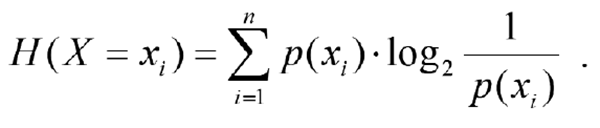
What exactly does this formula mean? The expression log₂ 1/p(x_i) is known as the Surprisal and usually notated as S(x_i). The Surprisal measures the degree of unpredictability or “surprise” of x_i happening. If the probability p(x_i) is very small, the surprise of x_i happening is very large. If, on the other hand, the value of p(x_i) is close to 1, the surprise of x_i happening is almost zero. In other words, the smaller the probability of an event is, the greater the surprise when it happens (a clear explanation is at plus.maths.org/information-surprise).

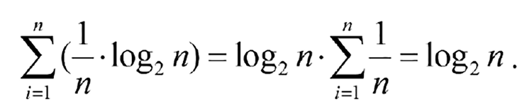
Basically, the Shannon entropy is the expected value of the Surprisal. It is the arithmetic mean of S(x_i) weighted by the probabilities p(x_i) of the events x_i with i = 1, 2, …, n. Of course, p(x₁) + p(x₂) + … + p(x_n) = 1. If all possible outcomes are equally likely to occur—that is, if p(x_i) = 1/n for i = 1, 2, …, n—then the Shannon entropy can be easily calculated. It is

But what if the possible outcomes are not all equally likely? If you experiment a bit using one of the several online Shannon entropy calculators (for instance, at www.omnicalculator.com/statistics/shannon-entropy or planetcalc.com/2476), no non-uniform distribution of probabilities appears to have an entropy greater than or equal to that of the uniform distribution. In fact, it can be proven that for all non-uniform distributions of Pr(X = x_i) with i = 1, 2, …, n, the Shannon entropy is smaller than log₂ n. A short proof can be found in the standard book about information theory, Elements of Information Theory by Thomas Cover and Joy Thomas.

In other words, unpredictability is at its maximum when all possible outcomes are equally likely for a finite number of possible outcomes. But by definition, nothing is more unpredictable than pure randomness. It follows that aleatory randomness and pure randomness coincide! The uniformity belief is a sound stochastic intuition after all, and not, as many assume, a biased notion of randomness.

As a matter of fact, the idea that randomness has no preference is common and of all times: The ancient goddess of chance, Fortuna, was depicted blindfolded.

But if the uniformity belief is a sound intuition, it cannot be held responsible for the illusion that switching doors makes no difference. Again, this looks like a dead end, but actually, there is still another possibility: the possibility that we are, in fact, dealing with not just two alternative possibilities but with more than two. But how can this be, with only two doors left? To resolve this apparent paradox, here’s a closer look at the mathematical background of the uniformity belief.

The Interchangeability Principle

The uniformity belief is embedded in aleatory randomness; that is, randomness that is generated by fair randomizers. A randomizer is called fair if it has no preference for any of its outcomes. But how do you know? The standard six-sided die, the archetype of a fair randomizer, is a useful example.

The fairness of a die has both a physical and a mathematical component. From a physical perspective, the roll of the die is fair if the die itself is not crooked and its roll is not manipulated. This physical fairness, however, makes little sense if the die is not already mathematically fair. What makes a die mathematically fair?

A standard die has the geometric shape of a cube. A cube is isohedral: (a) All six sides of a cube are identical in size and shape, and (b) any side A can be mapped onto any side B by rotation (and/or reflection) while leaving the cube looking exactly the same. In other words, all six faces of a die are completely interchangeable, and it follows that each face has an equal probability of occurring.

In general, the following rule can be formulated: If there are exactly N alternative possibilities that are completely interchangeable, they are equally probable, each with a probability of 1/N of occurring. The interchangeability principle lies at the basis of the conception of pure randomness. Think of an urn filled with exactly N marbles that are well-mixed. All marbles are the same in size and form, so they are completely interchangeable. It follows that in drawing a marble blindly from the urn, each marble has a probability of 1/N of being drawn.

In fact, the uniformity belief is the intuitive version of the interchangeability principle. It is, therefore, a basic stochastic intuition. In the Monty Hall problem, it operates as follows.

Two alternative possibilities seem to remain. Either the door we picked has the car behind it and the other door has the remaining goat, or vice versa. The two alternatives look identical. If someone switched the doors, you wouldn’t notice the difference. In other words, they are completely interchangeable. Therefore, both alternative possibilities have equal probability: Each door has a 50% chance of hiding the car.

However, we know this is wrong. Somehow, we have been fooled by the cunning Monty Hall. We have been led into the false belief that there are only two remaining alternative possibilities, when in reality there are still three. To understand how this is possible, return again to the example of the six-sided die.

The ‘Leibniz Illusion’

A die is fair if its six faces are completely interchangeable, but this also means that its faces are indistinguishable. After rotation, a cube looks exactly the same—as if nothing happened at all. To differentiate the alternative possibilities from each other, they must be labeled in some way. On a standard die, each of the six faces has a different number of dots, ranging from one to six. As a rule, the dots on opposite faces add up to 7.

Nature is blind to these labels, but when alternative possibilities are not labeled or somehow differentiated, humans can’t tell the difference between them. And when people can’t differentiate between two alternative possibilities, they tend to take them to be identical. A well-known example is the mistake made by the German mathematician and philosopher Gottfried Wilhelm Leibniz (1646–1716).

In a March 22, 1714, letter, Leibniz explained the basics of classical probability to the polymath Louis Bourguet, who was an ardent supporter of Leibniz’s philosophy: “The art of conjecture is founded on that which is more or less easy, or rather more or less feasible, for the Latin facilis (easy), derived from a faciendo (from what is to be done), literally means feasible: for example, with two dice it is as feasible to throw a twelve, as it is to throw an eleven, because both results can only be achieved in one way” (www.leibniz-translations.com/bourguet1714.htm).

Of course, this is not true. The sum of 12 can only be thrown in one way (6, 6), but the sum of 11 can actually be thrown in two ways (5, 6 and 6, 5). Instead of looking at all possible permutations, Leibniz looked only at the unordered combinations. That is a mistake that is still often made at an elementary level of efforts to understand probability.

Call the two dice D1 and D2. The sum of 11 can be realized as either 5 (D1) and 6 (D2), or 5 (D2) and 6 (D1). But if D1 and D2 look identical, as dice often are and are normally imagined to be, both these alternative possibilities will look exactly the same. As a result, we take them to be identical and conclude that there is only one possibility instead of two. It can, however, easily be shown that this is wrong just by giving the two dice different colors. Suppose D1 is colored red and D2 is colored blue. Then the illusion that the two outcomes are one and the same instantly disappears (unless, of course, you happen to be color-blind).

Others before and after Leibniz made and will make the very same mistake, but, as it happens, one of the principles of Leibniz’s own philosophy actually was the principle of the identity of indiscernibles. The illusion that two indiscernible alternative possibilities are identical can thus, with good reason, be called the Leibniz illusion.

Returning to Monty Hall, could we somehow have fallen victim to the same illusion that fooled Leibniz 300 years ago? Maybe labeling the three doors will clear things up, just like it did by labeling the two dice with different colors.

Labeling the Doors

Labeling the three doors is a quite natural thing to do, given that they are identical-looking. In the original reader’s question, the doors are simply labeled number 1, number 2, and number 3. It is assumed that each of the three doors has a 1/3 probability that the car is behind it. The contestant now picks door number 1. Next, the host opens a door with a goat behind it. In the original reader’s question, this is door number 3.

According to vos Savant’s critics, two alternative possibilities remain: either the car is behind door number 1 and the remaining goat behind door number 2 or the car is behind door number 2 and the remaining goat behind door number 1. The uniformity belief says that if two alternative possibilities remain, they have equal probability. vos Savant’s critics conclude that the probability that the car is behind the door picked by the contestant (door number 1) is now 1/2.

According to vos Savant, however, door number 1 has still a 1/3 chance of winning, but door number 2 has now a 2/3 chance. A typical argument in favor of vos Savant is the one given by Keith Devlin:

Suppose the doors are labeled A, B, and C. Let’s assume you (the contestant) initially pick door A. The probability that the prize is behind door A is 1/3. That means that the probability it is behind one of the other two doors (B or C) is 2/3. Monty now opens one of the doors B and C to reveal that there is no prize there. Let’s suppose he opens door C. (Notice that he can always do this because he knows where the prize is located.) You (the contestant) now have two relevant pieces of information:

1. The probability that the prize is behind door B or C (i.e., not behind door A) is 2/3.

2. The prize is not behind door C.

Combining these two pieces of information, you conclude that the probability that the prize is behind door B is 2/3. Hence you would be wise to switch from the original choice of door A (probability of winning 1/3) to door B (probability 2/3).

The 2/3 probability of winning the car if you switch doors is correct, but there is something fishy about Devlin’s argument: It contradicts the uniformity belief. The probability that the car is behind door A stays 1/3, but the probability that it is behind door B has increased from 1/3 to 2/3.

In his book Rationality, Pinker explains this change in probability by saying that probabilities are about our ignorance of the world. New information reduces our ignorance and changes the probability. In the Monty Hall dilemma, the all-seeing host provides this new information. But in truth, we will see, the information provided by Hall by opening one of the doors is purely hypothetical, so nothing changes.

vos Savant’s critics reason in accordance with the uniformity belief, but their answer is incorrect. Devlin’s answer is correct, but his argument contradicts a sound stochastic principle. Clearly, labeling the doors doesn’t seem to be of much help.

We appear to be caught in what the ancient Greeks called an aporia: a problem or dilemma that has no way out. But actually there is.

A Probability Shift

After labeling the three doors, it is assumed that the initial probability of the car being behind each of the three labeled doors is 1/3. Not only Keith Devlin, but the Wikipedia article about the Monty Hall problem says so: “before the host opens a door there is a 1/3 probability that the car is behind each door.” In fact, these prior probabilities are completely irrelevant.

Label the three doors A, B, and C. Let p(A) be the probability that the car is behind door A, p(B) that the car is behind door B, and p(C) that the car is behind door C. All three doors look identical, so each has a 1/3 chance of being picked by the contestant. The probability that the contestant will pick the door that has the car behind it is 1/3 ∙ p(A) + 1/3 ∙ p(B) + 1/3 ∙ p(C) = 1/3 ∙ (p(A) + p(B) + p(C)) = 1/3. Clearly, the he probability of each individual door hiding the car is not relevant at all.

This is only logical. The Monty Hall problem is not about the probability that the door you picked has the car behind it; it’s about the probability that you picked the door with the car behind it. The difference may seem subtle, but it is crucial. Compare picking a playing card from a deck. The issue is not whether the one card you picked has the ace of spades on its reverse side, but whether you picked the card with the ace of spades on its reverse side. Labeling the doors makes the focus shift from the relevant probability that we picked the door with the car behind it (P) to the irrelevant probability that the door we picked has the car behind it (P*).

What is P, the probability that you picked the door with the car behind it? Simple. There are exactly three doors. One of the three doors has the car behind it. All three doors look identical and therefore completely interchangeable. The interchangeability principle now tells us that P—the probability of picking the door that has the car behind—is 1/3.

But how does all this help us to escape from the aporia? Only two doors remain and therefore only two possible alternatives seem to remain: Either we picked the winning door or we picked the remaining losing door. In truth, however, there remain not two but three possible alternatives.

Hidden Labels

Labeling the three doors leads to a probability shift that only creates confusion, but how can we solve the Monty Hall problem without first labeling the three doors? As a matter of fact, the three doors are already labeled. How is that? Take the example of playing cards again. Each of the 52 cards is uniquely labeled by its color, suit, and rank. To randomly pick a card from a deck, these labels must, of course, be hidden. In exactly the same fashion, the car and the two goats can be thought of as the hidden labels of the three doors.

Name the door with the car behind it Door Car and the two doors with goats Door Goat 1 and Door Goat 2. Since their “labels” are hidden, the three doors look exactly the same. When you are asked to pick a door, there are three possible scenarios, each with a 1/3 probability:

1. You will pick Door Car.
2. You will pick Door Goat 1.
3. You will pick Door Goat 2.

After you pick a door, the host will open one of the other two doors, but only Door Goat 1 or Door Goat 2, never Door Car. Here’s what happens in each of the three possible scenarios:

1. If you picked Door Car, the host will open either Door Goat 1 or Door Goat 2.
2. If you picked Door Goat 1, the host will open Door Goat 2.
3. If you picked Door Goat 2, the host will open Door Goat 1.

Either Door Goat 1 remains and Door Goat 2 is eliminated, or Door Goat 2 remains and Door Goat 1 is eliminated. But since the two doors look exactly the same, we cannot say whether it is the door with Goat 1 behind it or the door with Goat 2 that remains, so we still have the same three alternative possibilities (the scenarios 1, 2, and 3), each having the same probability of 1/3. The information that is provided by the host opening one of the two doors you didn’t pick is purely hypothetical. Nothing changes at all, so P remains 1/3.

But we know that Door Car always stays in the game. Therefore, the probability that the other remaining door is Door Car must be 2/3. In other words, by switching doors, the probability P becomes 2/3.

Another way to make things clear is to uncover the “hidden labels” by giving each door a different color depending on what is behind it. Say Door Car is red, Door Goat 1 is blue, and Door Goat 2 is green. This would spoil everything. You just pick the red door and bingo! However, you happen to suffer from a very rare disease, known as achromatopsia: You are totally color-blind. As a result, the three doors look exactly the same to you, just as in the original show game. Now let the game begin.

First, you are asked to pick a door. There are three alternative possibilities, each with the same probability of 1/3:

1. You will pick the red door.
2. You will pick the blue door.
3. You will pick the green door.

Next, the host will open one of the two doors you didn’t pick, but only the blue one or the green one; never the red one. Here’s what happens in the three possible scenarios:

1. If you picked the red door, the host will open either the green door or the blue door.
2. If you picked the blue door, the host will open the green door.
3. If you picked the green door, the host will open the blue door.

Since you are completely color-blind, the information provided by the host opening one of the other two doors is purely hypothetical; nothing changes. The same three alternative possibilities remain, each still having a 1/3 probability. But since the red door always stays in the game, the other door will be the red door in two of the three alternative scenarios, so switching doors doubles probability P.

Monty Meets Leibniz

Using this “method of hidden labels,” we could find the correct answer without violating the uniformity belief. Using the same method, we can now also answer the question of why vos Savant’s critics (and a great many of her supporters) were wrongly convinced that only two alternative possibilities remain.

When the host opens a door with a goat behind it, there are two possibilities: The host opens either the door with Goat 1 behind it or the door with Goat 2 behind it. But we can’t tell whether he opens door Goat 1 or door Goat 2. The two doors are identical-looking, so the two alternative scenarios—either door Goat 1 remains closed and door Goat 2 is opened, or door Goat 2 remains closed and door Goat 1 is opened—look exactly the same.

When people cannot distinguish between two alternative possibilities, they tend to take them to be identical. This is what we called the Leibniz illusion. As a result, we simply conclude that one door with a goat behind it has been eliminated and one door with a goat behind it is left. Only two alternative possibilities instead of three now seem to remain: The door we picked has either the car behind it and the other remaining door a goat, or vice versa. But the uniformity belief says that if two alternative possibilities remain, they are equally probable. Clearly, chances are now 50-50.

In short, vos Savant’s critics were not blinded by the equiprobability bias, which is not a bias at all; they were fooled by the same illusion that once fooled Leibniz, one of the great mathematicians of all time. The same goes for all those who assert that the probability of the car being behind the other remaining door has increased from 1/3 to 2/3. And that’s not all: In doing so, they violate a sound stochastic principle as well.

To Resume

The Monty Hall problem seems to be a simple problem with a simple solution: Two doors are left—one with the car behind it and one with a goat behind it—so chances appear to be 50-50. But not according to Marilyn vos Savant. Her reply to a reader’s question that switching doors doubles your chances provoked a worldwide surge of disbelief, even among trained mathematicians. Luckily, as Falk remarked, the truth of mathematical propositions is not decided by a preponderance of votes. But why were so many people so deeply convinced that vos Savant was not only wrong, but even defied common sense?

The correct solution to the Monty Hall problem seems to contradict a strong and robust stochastic intuition that says that if exactly two alternative possibilities remain, they are equally probable. Falk referred to this intuition as the uniformity belief. This intuitive belief has its roots in the randomness that is generated by randomizers that were designed to be fair.

At first glance, there appears to be no reason why two alternative possibilities should always be equally likely. In cognitive psychology, the uniformity belief is therefore also known as the equiprobability bias. According to Pinker and other cognitive psychologists, the explanation for the surge of disbelief is that people were misled by this powerful bias.

Tempting as this explanation may be, it turns out to be false upon closer inspection. Using the concept of Shannon entropy, it can be shown that the uniform distribution entails maximum unpredictability. By definition, nothing is more unpredictable than pure randomness, so the uniformity belief is not a bias. As a matter of fact, it is an intuitive version of the interchangeability principle—a stochastic principle that lies at the basis of the concept of pure randomness. But if not the uniformity belief, what leads us astray?

When trying to solve the Monty Hall problem, people quite naturally label the three doors to be able to differentiate between them. Next it is assumed that each of the three doors has a prior probability of 1/3 that the car is behind it. These prior probabilities are, however, totally irrelevant. The Monty Hall problem is not about the probability that the door the contestant picks has the car behind it (P*), but about the probability that the contestant picks the door with the car behind it (P). This is the probability to focus on. The interchangeability principle tells us that P is 1/3.

Labeling the three doors only appears to create confusion. As a matter of fact, the doors are already labeled—according to what is behind them, just like playing cards. We named the door with the car behind it Door Car, one of the two doors with a goat behind it Door Goat 1, and the other Door Goat 2. When the host opens one of the two doors the contestant didn’t pick, there are two alternative possibilities: Either Door Goat 1 is eliminated and Door Goat 2 remains, or Door Goat 2 is eliminated and Door Goat 1 remains. However, we can’t tell the difference between these two alternative scenarios. They look exactly the same. As a consequence, we fall victim to what we called the Leibniz illusion: the illusion that two indiscernible alternative possibilities are identical.

After a door with a goat behind it is eliminated, only two alternative possibilities seem to remain: Either the door we picked has the car behind it and the other door a goat, or vice versa. The uniformity belief says that the probability that the car is behind the door that we picked (P*) is 1/2. But if we were asked which of the two doors with a goat behind it remains, we have to answer that we don’t know. It is either Door Goat 1 or Door Goat 2, so there remain not two but three alternative possibilities: We picked either Door Car, or Door Goat 1, or Door Goat 2.

By opening one of the two other doors, the host presents purely hypothetical information. It doesn’t change the 1/3 probability that the contestant picked Door Car (P), but because Door Car always remains in the game, the probability that the other remaining door is Door Car is 2/3.

vos Savant’s critics fell victim to the same illusion that deluded Leibniz and many before and after him: the illusion that two indiscernible alternative possibilities are one and the same. Apparently only two alternative possibilities remain. Therefore, chances must be 50-50. Any other distribution of probabilities contradicts the uniformity belief, and because the uniformity belief is a basic stochastic intuition, vos Savant’s counter-intuitive solution seems to defy common sense.

The Monty Hall problem may well be the best-known counterintuitive problem in probability, but it is certainly not the only one. The many counterintuitive results that can be found in probability have attracted much attention from cognitive psychologists, particularly those who endorse the heuristics and biases approach. In their attempts to explain these counterintuitive results in a psychological framework, though, they often tend to bite off more than they can chew. At the heart of most counterintuitive results in probability lie not cognitive biases or heuristics, but sound stochastic intuitions that are, however, misapplied. The mathematical anatomy of both the gambler’s fallacy and the Monty Hall problem testifies to this.

One question still remains to be answered that mathematics cannot explain. When Donald Granberg looked at the gender of vos Savant’s critics, he did not find a natural 50-50 proportion of men and women. Nearly nine out of 10 were men! How come? Would the same thing have happened, one wonders, if Marilyn vos Savant had not been a highly intelligent woman, but a man?

Further Reading

Bernoulli, J. 2006. The Art of Conjecturing, trans. by Sylla, E.D. Baltimore: Johns Hopkins University Press.

Cover, Th. M. and Thomas, J. A. 2006. Elements of Information Theory, second edition. Hoboken, NJ: John Wiley & Sons.

Falk, R. 1992. A Closer Look at the Probabilities of the Notorious Three Prisoners. Cognition 43, 197–223.

Falk, R., and Lann, A. 2008. The Allure of Equality: Uniformity in Probabilistic and Statistical Judgment. Cognitive Psychology 57, 293–334.

Granberg, D. 2014. The Monty Hall Dilemma: A Cognitive Illusion Par Excellence. Salt Lake City: Lumad Press. (Appendix A: Marilyn vos Savant’s Four Columns on the Monty Hall Dilemma; Appendix B: Two Letters to the Editor of The American Statistician by Steve Selvin.)

Laplace, P.-S. 1995. Philosophical Essay of Probabilities, trans. by Dale, A. I. New York: Springer Verlag.

Pinker, S. 2021. Rationality: What It Is, Why It Seems Scarce, Why It Matters. London: Allen Lane.

Tijms, S. 2022. The Mathematical Anatomy of the Gambler’s Fallacy, CHANCE 35(1), 11–17.

Vazsonyi, A. 2002. Which Door has the Cadillac. Adventures of a Real-Life Mathematician. New York: Writers Club Press.

vos Savant, M. 1996. The Power of Logical Thinking. New York: St. Martin’s Press.

About the Author

Steven Tijms studied mathematics, classics, and philosophy at Leiden University (The Netherlands). He is especially interested in the border area between mathematics and everyday life, and the history of mathematics. In classics, his focus is on Latin literature and Neo-Latin texts. He is a tutor of mathematics and the author of Chance, Logic and Intuition. An Introduction to the Counter-intuitive Logic of Chance (2021. Singapore/New Jersey/London: World Scientific).

Back to Top