
Probit and Wealth Inequality—How Random Events and the Laws of Probability Are Partially Responsible for Wealth Inequality

The distribution of wealth in the United States has grown more unequal in the last few decades. According to the U.S. Federal Reserve, the richest 1% of Americans now have about 15 times as much wealth as the combined wealth of the bottom 50%.
How rich or poor individuals become is partially determined by the level of talent they are born with; skills, education, and motivation they acquire; and effort and persistence they exhibit. The amount of support they receive from family, community, and government also plays a significant role, as do inheritance laws, tax laws, national and local employment swings, racism, sexism, and many other factors.
Wealth is also partially determined by random events. For example, some unlucky people must pay for the damage and lost wages imposed by severe weather (such as hurricanes Irma, Maria, and Harvey, which devastated parts of the South in 2017, and the freeze that crippled Texas in January of 2021); wildfires (like those that burned much of California in 2020 and choked the rest of the state); major illnesses and diseases (such as epilepsy, heart disease, and the COVID-19 pandemic); and accidents (automobile crashes, people falling off ladders, etc.). Others reap benefits from lucky breaks.
The laws of probability stipulate that even in a group of people who are identical in every way and are only subject to random costs and benefits, the distribution of wealth will be nudged toward taking the shape of the normal distribution’s cousin, the probit, with its very unequal allocation. And the larger these random costs and benefits are and the more frequently they occur, the more severe inequality will become.
To see this, consider two examples, each involving a simple game of chance.
Coin Flips
Imagine there are 100 people in a room and each one has $200. At the sound of a bell, each person flips a coin and if it lands heads up, they win that round of the game and gain a dollar. If the coin comes up tails, they lose a dollar. After playing 5,000 rounds of this (rather dumb) game, how rich would each of the people in the room be?
One might think that the wins and losses would balance out for every participant and each would end up with the same amount they began with; that is, $200. But that is not what actually happens. Instead, it is likely that, at most, only one or two participants would end up with exactly $200. Most would have a few dollars more or a few dollars less. Those who were really lucky, having flipped a significantly larger number of heads than tails, would have $250 or maybe even $300. Those who were especially unlucky would have $150 or even less.
It is conceivable that someone might flip 5,000 heads in a row and end up with $5,200, but this is extremely unlikely—the probability is 1/(0.55,000), which is approximately one chance in 101,505.
The overall results of a binary (only two possible outcomes) random event like this typically adhere to the principles of probability (the central limit theory) and produce a bell-shaped Gaussian distribution or normal distribution, as shown in Figure 1.
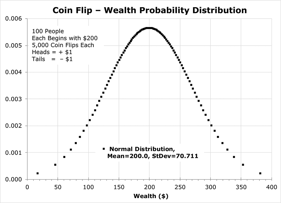
Figure 1. Probability distribution of wealth after 5,000 rounds of a simple coin flip game.
In this coin flip game, the curve peaks at $200, indicating that this is the most likely level of wealth, with about 0.57% of the participants ending up with this exact amount; $200 is also the average (mean) level of wealth among the 100 participants. Other levels of wealth are less likely the farther they are from this mean. The chances of ending up with exactly $50 or $350 is just 0.06%.
The standard deviation (which indicates the amount of variability in the results) is determined by the nature of the game and the number of rounds played. In this case, the standard deviation is 70.711 (see sidebar for the calculation). For the normal distribution, the values within one standard deviation from the mean account for 68.27% of the total, so 68 of the 100 participants would probably end up with between $130 and $270. Also, for a normal distribution, the wealth of 95.45% of participants would end up being within two standard deviations of the mean; that is, between $60 and $340.
This distribution is very different from the initial distribution in which every participant had the exact same wealth ($200). The mean is still the same ($200), but the standard deviation was 0 (no variation) initially and now, after 5,000 rounds of the game, has grown to 70.711.
If the 100 participants are sorted by their final wealth and their wealth is plotted versus each participant’s wealth rank order (which is also, since there are exactly 100 people, their percentile rank), the result is the quantile function or the inverse of the cumulative distribution function of the standard normal distribution—the probit. This curve, as seen in Figure 2, looks like a straight line sloping upward with asymptotic curls at both the richest and poorest ends (which reflect the way the normal distribution flares out at either side).
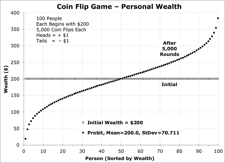
Figure 2. Wealth distribution after 5,000 rounds of a simple coin flip game.
Half of the participants end up with more than the initial $200 and half with less. On this curve, it is easy to see that 68% of the participants have wealth between $130 and $270, and 95% have wealth between $60 and $340. The richest person probably has about $382 and the poorest about $18.
Note how unequal this distribution is compared to the initial distribution in which every participant had the same wealth ($200). Through a totally random coin flip process, some people have become relatively rich and others relatively poor. Also note that the asymptotic curls at either end of this curve mean that the richest 1 percent (at the 99th percentile and greater) are significantly richer than those at the 95th percentile and the poorest 1 percent (at the first percentile or less) are significantly poorer than those at the fifth percentile. The laws of probability cruelly dictate that those who are particularly lucky become enormously richer than everyone else, and those who are especially unlucky. become notably poorer.
In this game, the more times the coin is flipped, the more unequal the distribution becomes. Figure 3 shows how the probit curve looks for other numbers of coin flips.
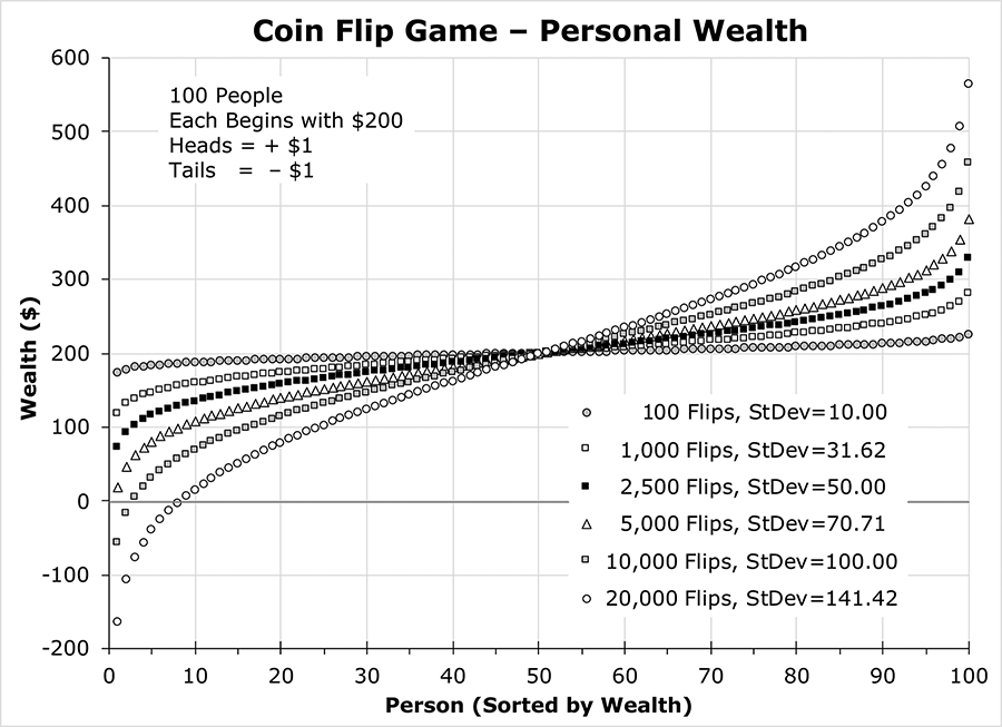
Figure 3. Wealth distribution for various numbers of rounds in a simple coin flip game.
After 100 coin flips, the distribution is almost flat, with the richest person having $226 and the poorest person having $174, just $52 less. But after 20,000 coin flips, the richest person has $564 and the poorest person has –$164 (they owe money), which is $728 less than the richest.
This simple coin flip game involves only a trivial amount of money—just a few dollars in each round—and requires thousands of rounds before any significant inequality develops. But what if the stakes in each round were much higher (like they are in many real-life random events, such as whether or not your house is hit by a tornado)?
Coin Flip Plus Die Roll to the Sixth Power Game
Imagine another room with 100 people, but this time, each one has $200,000 initially. At the sound of a bell, each person flips a coin and rolls a die. If the coin lands heads up, they win that round of the game and gain an amount equal to the number of dots on the die raised to the sixth power; that is, multiplied by itself six times. For example, if they roll a 3, they collect 36 = $729; if they roll a 6, they receive 66 = $46,656. If the coin comes up tails, they lose an equivalent amount. In this game, rolling a 1—whether winning or losing—does not affect a person’s wealth very much, but rolling a 6 makes a big difference.
Because the stakes in this game are much higher, the people in this room only play 10 rounds of this game. How rich would each become?
This game would also produce a normal probability distribution, but with a mean of $200,000 and a standard deviation of $63,747.36. The wealth distribution among the 100 players would again be a probit, as shown in Figure 4.
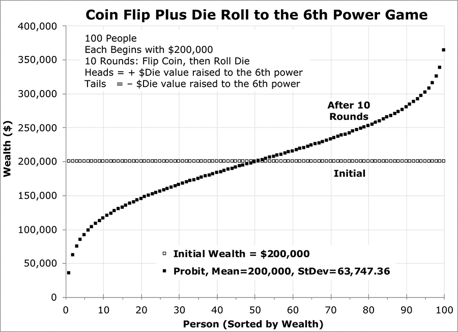
Figure 4. Wealth distribution after 10 rounds in a game of coin flip plus die roll to the 6th power.
After just 10 rounds of this high-stakes game, the richest person has gained $164,202 and now has $364,202. This is 10 times as much as the poorest person who has lost $164,202 and now has only $35,798.
Since the probit curve is asymptotic on both sides, if there were 100 million people in the (very crowded!) room instead of 100, the asymptotic values would be even more extreme at the top and bottom, as Figure 5 shows. The richest person (at the 99.999999th percentile) would have $565,319, which is $730,638 more than the poorest person (at the 0.000001th percentile) with –$165,319.
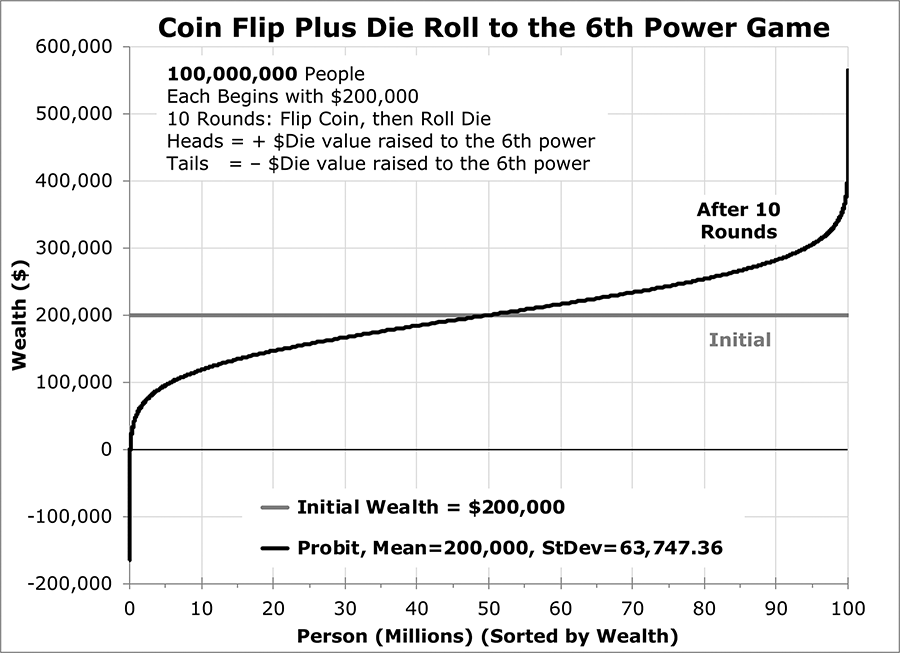
Figure 5. Wealth distribution after 10 rounds in a game of coin flip plus die roll to the 6th power with 100 million players.
The richest person may look down arrogantly on the poorest person, but again, this drastic difference in fortunes is not caused by differences in talent, skill, experience, effort, or persistence, but is simply due to random luck and the laws of probability. In this game, just a few unfavorable flips of a coin and rolls of a die can wipe out most of someone’s wealth.
Calculating the Standard Deviation of a High-Stakes Coin Flip Game
Sequentially flipping a coin and then rolling a die produces 12 possible outcomes, each equally probable (1/12 = 0.08333 probability each). But the earnings of these outcomes are very different: positive for the coin flips that result in heads and negative for those that result in tails, with the amount earned (or lost) equal to the number of dots on the die raised to the sixth power.
Table 1 shows how to calculate the expected value for each outcome, which is the probability of each outcome times its earnings (x times P). In the last column, it shows the variance for each outcome which is the expected value times the probability of that outcome (x squared times p). The sum of the 12 variances gives the overall variance for one round of the game = $406,372,619.17. The variance for 10 rounds is this value multiplied by 10. The standard deviation is then the square root of this amount and equals $63,747.36.
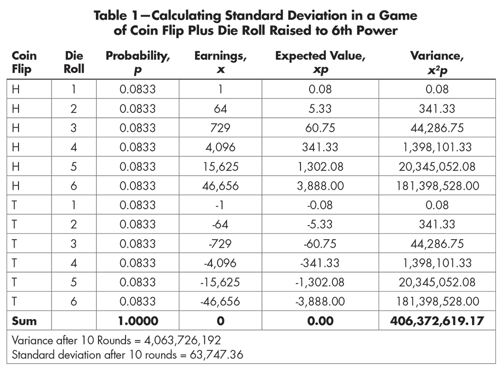
Table 1—Calculating Standard Deviation in a Game of Coin Flip Plus Die Roll Raised to 6th Power
Table 2 shows the standard deviation for different numbers of rounds of this game. Even for a single round in this high-stakes game, the standard deviation is $20,158.69. After 10 rounds, the standard deviation has grown over three times larger to $63,747.36 and the level of wealth of those who are very lucky separates significantly from those who are very unlucky.
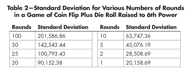
Table 2—Standard Deviation for Various Numbers of Rounds in a Game of Coin Flip Plus Die Roll Raised to 6th Power
Rugged Island
The results of these two simple games of chance are interesting, but do they provide any useful insight about the actual reality? Perhaps so.
In a long life, every person is likely to experience a few events that randomly increase or decrease their wealth by a significant amount. For example, wildfires and severe weather (earthquakes, tornadoes, hurricanes, floods, high winds, blizzards, hailstorms, heat waves, etc.), serious illness (cancer, diabetes, heart disease, deadly viruses, etc.), and major accidents (auto, workplace, household, etc.) usually impose very large economic expenses on those who must endure them. These “acts of God” are also mostly beyond anyone’s control and seemingly strike people at random. Over the course of a life, most people are probably subjected to at least one of these costly, random circumstances and some take the full brunt of several.
A visit to Rugged Island, one of the fictitious Chancy Islands (a set of computer spreadsheet models; see www.chancyislands.org), can show the economic impact that these random events might have. The Chancy Islands are unusual in that every island has exactly 500 households and each household is identical, consisting of two adults who live in a house they own outright (no mortgage) worth $200,000 and who have cash savings of $5,000. Every household has exactly the same annual income ($60,000) and the same annual ordinary expenses ($54,000), which are similar to the average income and expenses of a typical middle-class American household. Each household is also subjected to severe illness, weather, and accidents that cause them to incur random amounts of extra expenses and catastrophic losses totaling, on average, $6,000/year, but varying from $0/year to more than $200,000/year—amounts that are also similar to those affecting American households.
The amounts of both the extra expenses and catastrophic losses are calculated randomly for each household for each year by feeding a computer-generated random number into an exponential decay function that decays rapidly. Amounts close to the maximum amount ($40,000 for extra expenses and $200,000 for catastrophic losses) strike only a few households each year; most households incur little or no expense in most years.
Because there are no differences in talent, education, skills, or effort on Rugged Island nor any of the many other economic factors in the complex real world, it is possible to get a sense of the impact on typical households of severe earthquakes, wildfires, weather, illness, and accidents striking at unpredictable times and imposing random expenses.
The result: As Figure 6 shows, significant wealth inequality develops after 50 years.
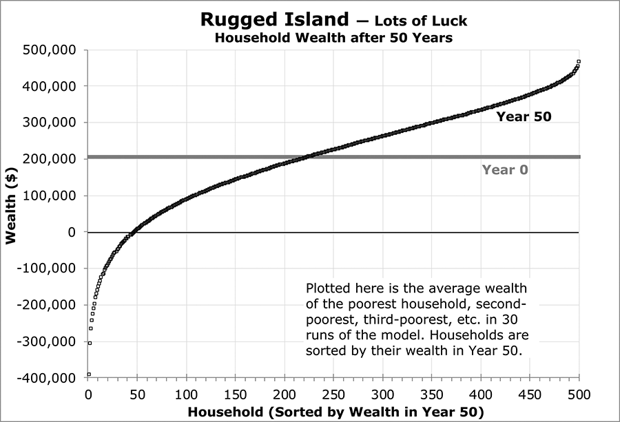
Figure 6. Wealth distribution on Rugged Island (computer model) in Years 0 and 50.
The shape of this curve is similar to a probit—with an upwardly-sloping straight line in the middle and asymptotic curls at the ends—but is not the same. Like the two games of chance described above, the wealth distribution on Rugged Island is shaped only by random events, but this process is much more complex than a simple coin flip or dice roll and produces a much more complex wealth distribution. Also, unlike the games of chance described above, the random events on the Chancy Islands only impose variable losses—all gains are constant.
Although Rugged Island began (in Year 0) with a uniform wealth distribution (every household started with $205,000 in wealth), 20 households have more than doubled their wealth after 50 years, while several others have sunk to a negative wealth of less than $300,000. This severe inequality was caused solely by a series of random events.
Conclusion
These examples show that any society subject to random economic costs and benefits will develop some wealth inequality produced solely by the laws of probability. A large number of small random economic fluctuations or a small number of large fluctuations can cause significant inequality, and that inequality will tend to be most extreme at the very top and very bottom of the wealth distribution (reflecting the asymptotic curls at either end of the probit curve). Even if every person in a society is identical and acts in exactly the same way, some wealth inequality will still develop simply from events like earthquakes, wildfires, severe weather, major illness, and accidents that strike people randomly and are beyond anyone’s control.
If a society values fairness, then it must, in some way, mitigate the wealth inequality caused by these natural events and not let the whims of luck and the quirks of probability bestow vast riches on a few people and dire poverty on others.
Further Reading
Goldstein, Dan. 2017. Counterintuitive problem: Everyone in a room keeps giving dollars to random others. You’ll never guess what happens next. Decision Science News.
About the Author
Randy Schutt is a retired engineer. He earned BS and MSME degrees from Stanford University and is a current explorer of the Chancy Islands.


