
Toward Reducing the Possibility of False-Positive Results in Epidemiologic Studies of Traffic Crashes

Large databases, such as the U.S. Fatality Analysis Reporting System (FARS), are often used to study factors that influence traffic crashes that result in injuries or deaths, and how such events may be affected by human activities or environmental conditions. This genre of epidemiologic research presents considerable study design challenges, since crash rates vary by season, day of the week, and time of day.
To minimize the effects of these extraneous factors, many studies use a double-control matched design as laid out by Redelmeier and Tibshirani in the Journal of Clinical Epidemiology in 2017. This design identified the particular days (or portions of a day) in which the condition/factor of concern was present. The concern might relate to a national election or holiday, or Super Bowl Sunday, or the change to/from daylight savings time (DST). For each such day of concern, and for each year for which data are available, two comparison days—seven days before and seven days after—are identified. The notation for the counts of interest on these three days is shown in Figure 1.
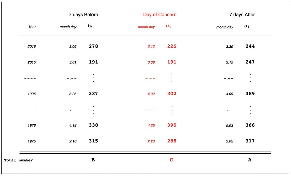
Figure 1. Counts of people involved in a traffic accident with at least one fatality.
The statistical methods used to convert the summed counts (C, B, A) in Figure 1 into inferential statistics typically follow those laid out by Redelmeier and Yarnell in CHANCE (2013). The estimand—the comparative parameter to be estimated—is the rate ratio (RR), namely the ratio of the expected rate of interest for the day of concern to the expected rate of interest for the (matched) control days. The estimator of the RR is the ratio of C to (A + B)/2 (under the assumption that the denominator is constant across all three days). Other estimands, such as the rate difference, may also be of interest.
Figure 1 illustrates the -7/+7 study design using the FARS data set, and our notation. The day of concern is the Monday immediately after the change to Daylight Savings Time. In any given year i, we denote by ci, bi, and ai—the relevant count on the Monday of concern, the Monday before and the Monday after. Their sums over all years studied are denoted by C, B, and A. Here, as is the case in many reports, the counts refer to the numbers of people involved in a traffic crash with at least one fatality, but the numbers of cars involved in crashes could also be considered (as seen later).
The null hypothesis is that the expected count of interest per day (i.e., the rate) on days of concern does not differ from the expected counts of interest per day for the pair of “control” days (i.e., that the RR parameter equals 1). The null hypothesis is typically tested by calculating the binomial probability that C or more of the total (B + C + A) would occur on the days of concern, assuming an expected proportion of 1/3. A confidence interval (CI) for the RR is obtained using the same binomial model. This interval can be calculated exactly or, since C, B, and A are usually large, as the anti-log of a z-based CI that uses the standard error (SE) of the log of the point-estimate.
The SE is computed as (1/C + 1/[A+B])½. The same p-value and the same CI would be obtained if C and (A + B) were treated as two Poisson random variables. As shown by Clayton and Hills (1993), the SE can be derived by fixing (conditioning on) their sum, and treating C as a binomial random variable with expected proportion RR/(2+RR), or by an unconditional argument.
This SE, involving just the three observed totals, C and (A + B), and the CI derived from it, is too narrow when applied to traffic-related counts of total crashes involving at least one fatality, or of the number of individuals involved, injured, or dying in such crashes. It leads to too many empirical rate ratios being declared statistically significant, and to overly precise SEs.
Orientation: The Rutherford Standard Error
To understand why this SE is too narrow, it helps to consider an example of a Poisson process. Imagine counting the scintillations (flashes of light) produced by the decaying products from a radioactive source in a laboratory setup resembling that used by Rutherford and colleagues in 1910. The experiment involved 42 separate occasions, each with a duration of 3 minutes.
On each occasion, the distance from the source to the target is fixed at X during the first and third minutes, and made 5% shorter during the second minute. Just as in Figure 1, the scintillation counts are denoted in the successive minutes of each occasion i as bi, ci, and ai, and their sums over all occasions as B, C, and A. Suppose that, from one occasion to another, the distance from the source target may vary.
The purpose is to use these data to estimate the ratio of the radioactive intensity detected when the source-distance is 0.95X rather than X. The estimand is the Rate Ratio parameter RR, and the data yield an estimate of RR. As Rutherford and colleagues were able to show, both theoretically and empirically, the “control” counts—bi and ai—arise from a Poisson distribution with a common (but unknown) mean mi, and ci arises from a Poisson distribution whose mean is RR times mi. Because of the between-occasion variation in the strength of the source, the unknown means (mi and RR times mi) vary from occasion to occasion.
Nevertheless, each within-occasion ratio ci / [(ai + bi)/2] can be used to estimate the common RR. Moreover, the estimator of RR is the ratio of C to (A + B)/2, and the expression (1/C + 1/[(A + B)])½ provides an appropriate SE for its log. However, this SE only holds if, on each occasion, the bi, ci, and ai counts follow the two Poisson laws just described. It would be too narrow if, within some occasions, the strength of the source is allowed to vary from minute to minute. This SE formula can be referred to as the Rutherford SE, to emphasize that its accuracy can only be guaranteed within these controlled laboratory conditions.
In traffic crash epidemiology, a large number of environmental and social factors cannot be controlled (or adequately controlled for) by the investigators. Thus, one would not expect the counts from the two comparison days in the same year to arise from a Poisson distribution with the same mean even if these two days are on the same day of the week and just 14 days apart.
FARS data can be used to demonstrate empirically that the pair of counts from days just 14 days apart in the same year do not share the same mean and variance, to identify 1,094 non-overlapping pairs of days that were 14 days apart, and to derive the corresponding bi and ai counts (of the individuals involved in car crashes that have at least one fatality) for these pairs (Figure 2). For each pair, we calculated the within-pair difference bi–ai and converted it to a Z-value, assuming that for any particular pair, the two counts arose from two independent Poisson distributions with the same expected value.
Under this assumption, which is at the core of the Rutherford SE used by Redelmeier and Yarnell, the resulting histograms should resemble standard Gaussian distributions. However, Figure 2 provides considerable evidence of “extra-Poisson” variation in the bi and ai counts for the two comparison days in the same year. The observed Z-values have a distribution that is two to three times wider—flatter relative to the familiar bell shape—than Rutherford would have observed within his (bi ai) pairs (Figure 2). Thus, even though the expected ratio under the null is 1:2 in the -7+7 design, it does not automatically follow that the observed split of the (bi + ci + ai) count in any one year, or in the overall (B + C + A) count, between the two types of days should follow a binomial distribution. Instead, it will exhibit extra-binomial variation.
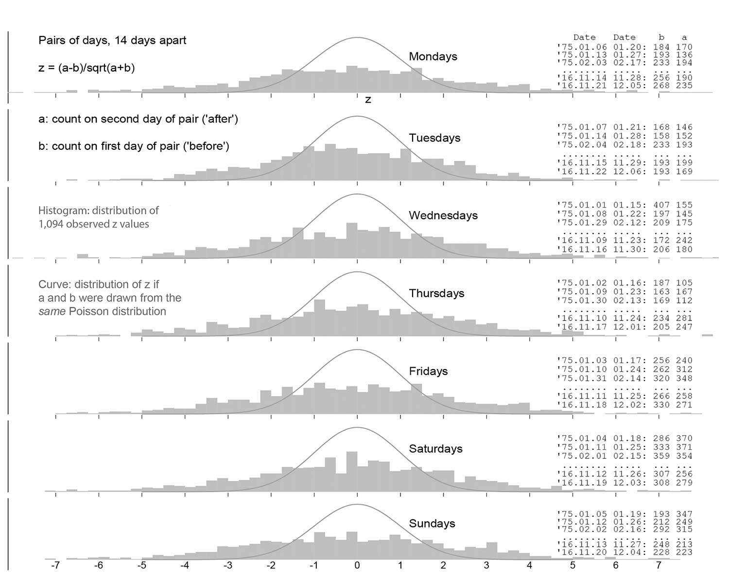
Figure 2. Extra-Poisson variation in the counts of individuals involved in car crash with at least one fatality on two comparison days 14 days apart in same year (FARS, 1975–2016). Observed z-values have a distribution that is two to three times wider than that predicted by the prevailing model used to calculate an SE for the log(RR).
There is additional proof that using the Rutherford SE in double-control matched designs of traffic-related counts produces confidence intervals that are too narrow, and there also are other existing methods (extra-binomial and bootstrap-based) for calculating the SE for the log(RR) estimate. These do not make the restrictive Poisson assumptions that would only be satisfied in a laboratory setting.
Three alternative data-based methods (jackknife, permutation, and split-halves) and two regression-based methods (quasi-Poisson and negative binomial) can be proposed.
Finally, the seven alternative SEs are more conservative and more realistic than the Rutherford SE. All of the code and data to reproduce the analysis can be found here.
Standard Errors and Their Impact on Statistical Inference of Log Rate Ratios
Eight methods may be used to compute the SE of the log(RR): the Rutherford SEs, extra-binomial, jackknife, bootstrap, permutation method, split-halves estimate, negative binomial regression, and quasi-Poisson regression. Box 1 provides more detail for each method.
To compare the performance of these methods, we applied each method to the calculation of the SE of the log(RR) comparing a day of concern and two comparison days a week apart, for each of the 365 possible days of concern in the calendar. We used the FARS data and repeated this analysis, each time with 42 triplets (one for each year from 1975 to 2016) and excluding February 29 from all analyses.
The eight methods can also be applied to three simulated data sets. The three simulated data sets were derived from fitted values of a quasi-Poisson regression applied to the count of all individuals involved in a crash with at least one fatality in the FARS data. This measure is conventionally used in the literature.
The model had 63 parameters, one for each year (42), month (12), day of the week (7), January 1 (1), and July 4 (1). These fitted values were then used as the means for each day of the year for the simulations.
The first simulated data set has no extra-Poisson variation, the second has half the extra-Poisson variation as the FARS data set, and the third has double the extra-Poisson variation as the FARS data set. This resulted in a total of 11680 (8 x [3 + 1] x 365) SEs for the log(RR): one for each of the 365 days, for the eight methods, over the FARS data and the three simulated “data sets.” The distribution of SE estimates, as well as the median and interquartile range (IQR) for each method, are presented as boxplots in Figure 3.
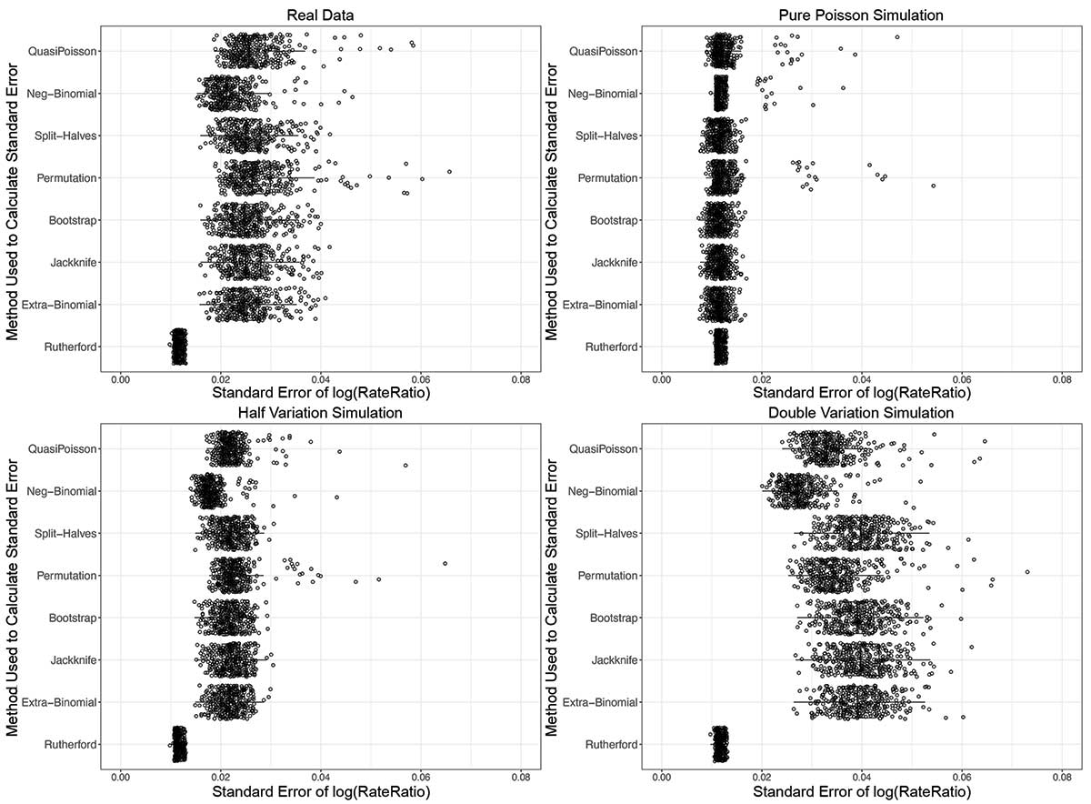
Figure 3. Boxplot of 365 SEs obtained using each proposed method for calculating SEs for log(RR). SEs are from: real world data (top left); pure Poisson simulated data (top right); simulated data with half the variation of real data set (bottom left); and simulated data with double the variation of real data set (bottom right). Rutherford SE is the only method that does not demonstrate a change in variability among the four conditions. Median and IQR for Rutherford SE are consistently smaller and less variable than the other SEs.
For the FARS data, the smallest median and IQR for any of the methods tested were from the Rutherford SE: median = 0.011 and IQR = 0.001. The next-smallest median and IQR were for the extra-binomial, bootstrap, jackknife, and split-halves methods, which all had medians of 0.025 and IQRs of 0.005. The most-conservative was the permutation method, which had a median of 0.026 and an IQR of 0.006.
On average, the IQR for the other methods was five to six times larger than for the Rutherford method, and the medians were more than double (Figure 3).
For the first simulated data set with no extra-Poisson variation, all the SE methods tested had roughly the same median and IQR (Figure 3). Notably, the median (0.011) and IQR (0.001) from the Rutherford SE were similar in the simulated Poisson data set as in the FARS data, despite the fact that the simulated, purely Poisson data set has no extra-Poisson variation and the FARS data have a considerable amount.
The second simulated data set, with half the extra-Poisson variation, had medians and IQRs that changed for all the methods relative to the amount of variation, except for the Rutherford method (Figure 3). In the simulated data set with double the amount of extra-Poisson variation, all the methods again responded to the doubling in variance, with the exception of the Rutherford method (Figure 3).
These simulations demonstrate that the Rutherford SE is systematically smaller and less variable than the seven other methods, and fails to incorporate extra-Poisson variation.
To examine the impact of these different methods for calculating SEs on statistical inference, we used the FARS count of individuals involved in car crashes to compute a Z-value for every day of the year for each SE method.
A Z-value measures how many standard deviations an estimate is from the null, assuming the null hypothesis is true. Z-values greater than 2 or less than -2 were considered as “statistically significant,” using a conventional threshold for alpha set at 0.05.
Figure 4 reports a representative sample of these results as heat calendars, with each day representing the Z-value estimated using 42 years of pooled data. Each graph uses the same color scale to display the intensity of the Z-values. The positive end of the scale is shown in dark red with a maximum value of 40. The negative end of the scale is in dark green with a minimum value of -25.
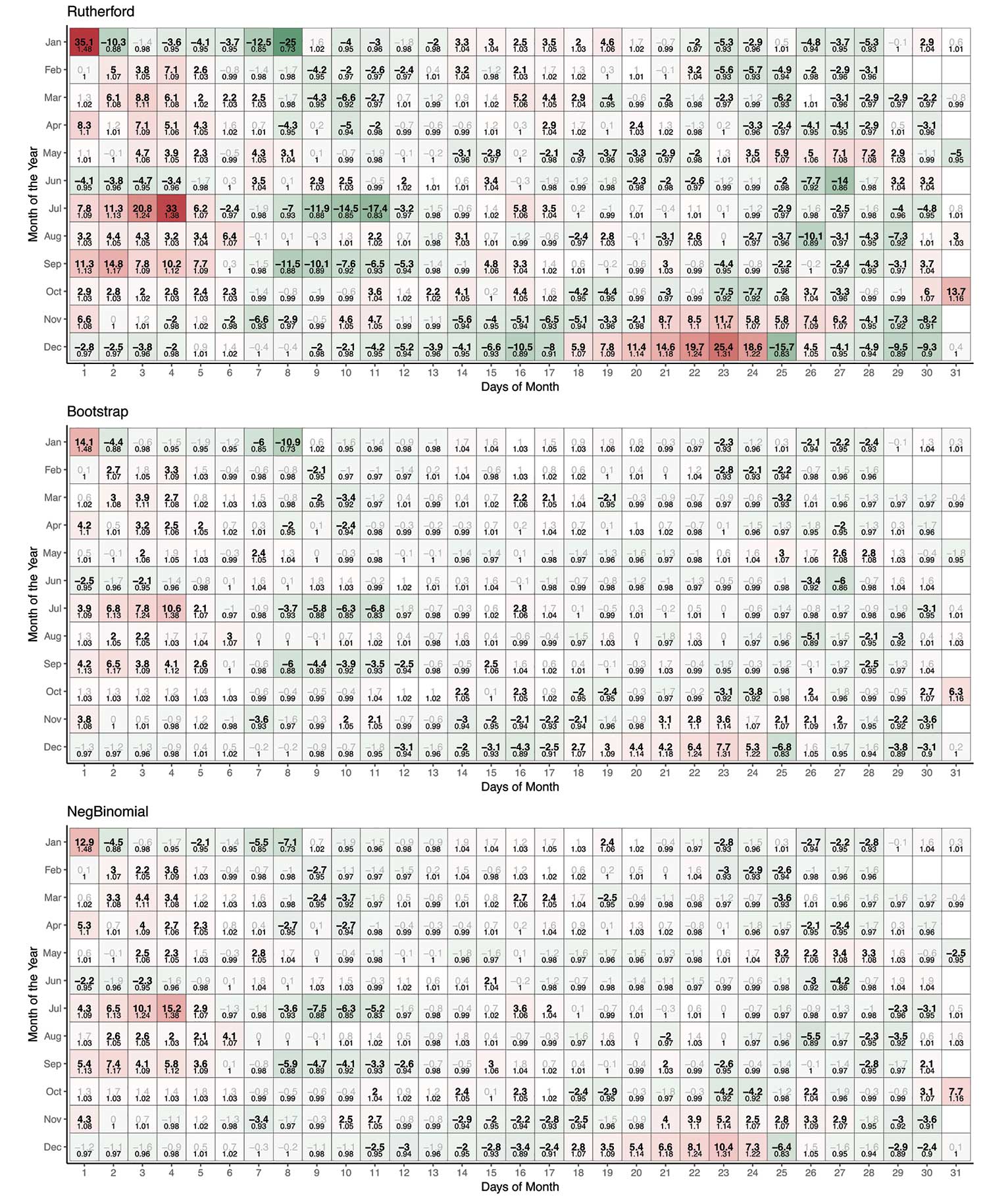
Figure 4. Heat calendars showing the Z-values produced by selected SE methods, for each day of the year. Z-values above 2 or below -2 are in bold and in black; non-significant values are grayed out. Point estimates of rate ratio are shown below Z-value for reference. The Rutherford calendar, along with two representative calendars (Bootstrap and Negative Binomial) of the seven other methods, all had similar heat calendars, except for the Rutherford calendar, which had more extreme values than other methods and has more days considered to be “statistically significant.” Heat calendars for all the methods can be found in osf repository.
The maximum and minimum were determined by taking the maximum and minimum Z-value among the 2,920 estimates and rounding them to the nearest base 5 number. In addition, Z-values that were considered significant at alpha = 0.05 were shown in bold, while non-significant values were shown in gray to provide a visual contrast.
Not surprisingly, it is evident from the heat calendars in Figure 4 that the Rutherford calendar has more “significant” days than any of the other two calendars, and in general, the Z-values are larger in absolute value. The calendars for the bootstrap and negative binomial methods are similar to each other and show less intensity relative to the Rutherford method. The calendars for the other five alternative methods strongly resemble the non-Rutherford calendars in Figure 4 (additional calendars can be found here).
In total, the Rutherford SEs led to 225 days out of 365 being incompatible with the null (i.e., an absolute Z-value greater than or equal to 2), while the other methods yielded roughly half that number (Figure 4). This is not surprising, given the results in Figure 2: The overly narrow nature of the Rutherford SEs leads to many more “statistically significant” results, largely by failing to account for the extra-Poisson variation that is present in the numbers of individuals who are involved in a traffic crash with at least one death that occurs on the same day of the week but just seven or 14 days apart in the same year.
Counting Individuals in Crashes vs. Number of Cars in Crashes
So far, the focus has been on the number of total individuals involved in traffic crashes with at least one fatality. Clearly, the multiplicity is one of the reasons for the greater-than-Poisson noise. However, the greater-than-Poisson noise is still evident, even when any multiplicity is removed and only the number of cars in crashes involving at least one fatality (Figure 5) are counted.
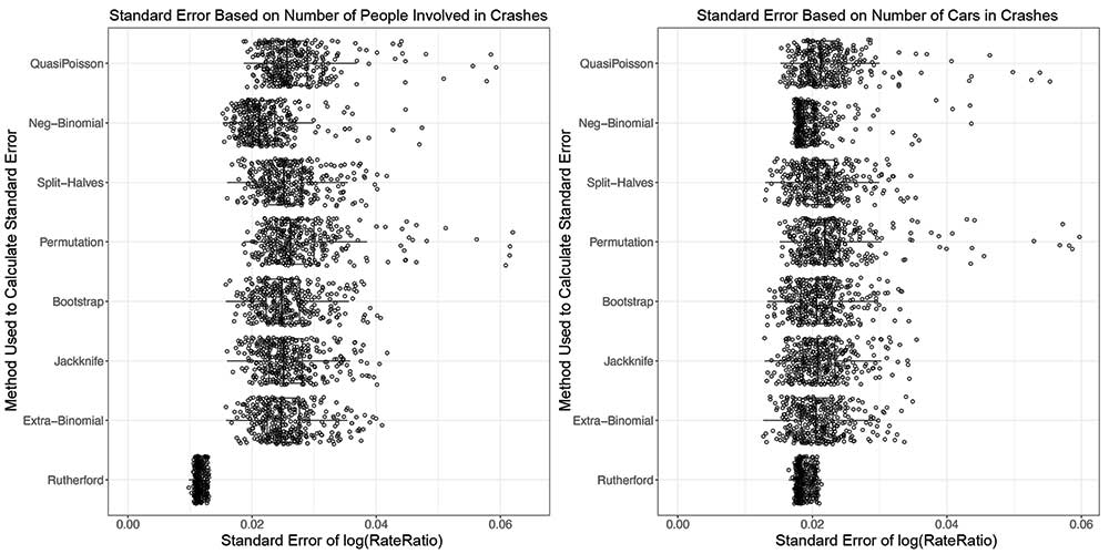
Figure 5. Boxplots showing variation in SEs for methods applied to FARS data set that includes all people involved in crashes with at least one fatality (left), and results for methods applied to FARS data set that only considers number of crashes with at least one fatality. The Rutherford SE is less variable than the other methods in both data sets.
The reason goes back to the large number of factors that affect the variation in the numbers of fatal crashes on the same day of the week, but two weeks apart, in a wide geographical area. The count-triplets recorded by Rutherford emanate from the same amount of inanimate source material (the alpha decay of an atom), observed over 3 adjacent minutes in one secluded laboratory. The narrow SEs derived from this ideal model are not appropriate for epidemiologic studies of fatal traffic crashes.
In Conclusion
This study compared eight ways to calculate SEs for the log(RR) that contrast rates of traffic-related events using the “double control” design, and examined their impact on statistical inference. The results demonstrate that the currently used method (which only holds under strict Poisson assumptions) does not account for the demonstrable extra-Poisson variation in the numbers of persons or crashes on days that are just 14 days apart but on the same day of the week. These methods lead to an excess of “statistically significant” days.
This study also demonstrates seven alternative methods for calculating standard-errors that do not suffer from this problem and should be used instead. Data-based SEs (Jackknife and Bootstrap) are more appropriate than overly tight SEs based on statistical models that may not mimic actual variation. A switch from overly tight, good-only-in-the-laboratory, model-based SEs to empirical (robust) SEs would lead to improved statistical inference in this field of research.
Further Reading
Clayton, D., and Hills, M. 1993. Statistical methods in epidemiology. Oxford, UK: Oxford University Press. Chapter 13.
Redelmeier, D.A., and Yarnell, C.J. 2016. Can tax deadlines cause fatal mistakes? CHANCE 16;26(2):8–14.
Rutherford, E., Geiger, H., and Bateman, H. 1910. LXXVI. The probability variations in the distribution of alpha particles. The London, Edinburgh, and Dublin Philosophical Magazine and Journal of Science. 20 (118):698–707. doi: 10.1080/14786441008636955.
Harper, S., and Palayew, A. 2019. The annual cannabis holiday and fatal traffic crashes. Injury Prevention 28:injuryprev-2018.
Weast, R. 2017. Temporal Factors in Motor Vehicle Crashes—10 Years Later. Arlington, VA: Insurance Institute for Highway Safety.
BOX 1: Methods to Compute SE of log(RR)
1. Rutherford: Staples and Redelmeier illustrated the SE of the log(RR) (in CHANCE. 2013). The log(RR) is estimated as log{C / ([A + B] / 2)}, where C is the total number of instances (of the entity being counted) in the n days of concern C = Σci; where B is the total number of instances on the “before” control days, B = Σbi; A is the corresponding sum, Σai, of the counts in the n “after” days and i is the index of the years over which the counts are summed. SE (log [![]() ] = (1/C + 1 / [A + B])½. It is derived by assuming that C and B + A are two Poisson counts, with expectations μnull and 2 × μnull × RR respectively. With this assumption, the single random variable obtained by conditioning on their sum, i.e., C | (C + A + B), has a binomial distribution with parameters ′n′ = C + A + B and π = RR / [RR + 2].
] = (1/C + 1 / [A + B])½. It is derived by assuming that C and B + A are two Poisson counts, with expectations μnull and 2 × μnull × RR respectively. With this assumption, the single random variable obtained by conditioning on their sum, i.e., C | (C + A + B), has a binomial distribution with parameters ′n′ = C + A + B and π = RR / [RR + 2].
2. Extra-binomial: This SE for the log(RR) estimator explicitly uses the n matched (by year i) pairs of counts, {c1,[a1 + b1]} to {cn,[an + bn]}. It allows for the strong possibility that even if the RR were truly 1, the counts for the three days in the same year have considerably greater-than-Poisson variation, and thus that each ci | (ci + ai + bi) follows an extra-binomial distribution. Instead of a model-based SE that assumes merely binomial variation, this SE is based on the empirical (actual) year-to-year variations in the proportions of the instances that occur on the day of concern. It is obtained by fitting an intercept-only logistic model to the n pairs of counts, and then applying the “sandwich” (robust, “empirical”) estimator of the SE (see R code).
3. Jackknife: This SE also explicitly uses the matching. Systematically excluding each triplet in turn provides the n jackknife estimates log[̂![]() ][-1] to log[
][-1] to log[![]() ][-n], where the subscript denotes the deletion of the ith data point i = 1,…,n. Let di denote the amount by which the ith of these differs from loĝ
][-n], where the subscript denotes the deletion of the ith data point i = 1,…,n. Let di denote the amount by which the ith of these differs from loĝ![]() , the jackknife SE for log[̂
, the jackknife SE for log[̂![]() ] is calculated as SEjackknife = {n-1⁄n × Σdi2}(½).
] is calculated as SEjackknife = {n-1⁄n × Σdi2}(½).
4. Bootstrap: This SE also explicitly uses the n triplets of matched counts. It creates several data sets, each one containing n triplets sampled with replacement from the indices 1 to n. The bootstrap SE is calculated as the standard deviation of the several estimates of log[![]() ] obtained from these different perturbations of the original data set.
] obtained from these different perturbations of the original data set.
5. Permutation: This SE also explicitly uses the matching. Within each triplet, one of the three days is chosen at random to serve as the day of concern, with the remaining two serving as the “reference” days. A value of log[![]() ] is calculated. This process is repeated several times and the standard deviation of the several estimates serves as the (null) SE. Under the null, there are three choices for the possible day of concern for each of the 42 years, so there are 3 to the power of 42 (1.09e + 20) possible rate ratios. Since it takes too long to generate them all, they are sampled instead.
] is calculated. This process is repeated several times and the standard deviation of the several estimates serves as the (null) SE. Under the null, there are three choices for the possible day of concern for each of the 42 years, so there are 3 to the power of 42 (1.09e + 20) possible rate ratios. Since it takes too long to generate them all, they are sampled instead.
6. Split-Halves: This SE also preserves the matching. A random n/2 of the n triplets are randomly selected. A log[![]() ]is calculated from the resulting C and (A + B)/2, and subtracted from the log[
]is calculated from the resulting C and (A + B)/2, and subtracted from the log[![]() ] obtained from the remaining half. This process is repeated several times, and the standard deviation of the several differences computed. The SE is obtained by multiplying this standard deviation by 1/2 if n is even, and by a slightly smaller factor if n is odd (see R code).
] obtained from the remaining half. This process is repeated several times, and the standard deviation of the several differences computed. The SE is obtained by multiplying this standard deviation by 1/2 if n is even, and by a slightly smaller factor if n is odd (see R code).
7. Negative Binomial: This SE is obtained by regressing the 3n observed counts on n + 1 regressors, namely an indicator variable of the day of concern, plus a factor of length n representing n separate intercepts—one per triplet—and using the generalized linear regression function shown in the code. The output consists of the log(RR) estimate and its SE, together with the n fitted intercepts and their SEs, along with the fitted extra-Poisson parameter θ. The smaller the θ value, the greater the extra-Poisson variation, and the SE of interest. This regression can be seen as model-based—rather than actual—matching: For triplet number 5, say, conditional on its own separate intercept μ5, the two reference counts follow a negative binomial distribution with mean μ5 and variance μ5 + μ52 / θ, and the count on the day of concern follows a negative binomial distribution with mean RR × μ5 and variance RR × μ5 + (RR × μ5)2 / θ.
8. Quasi-Poisson: The SE is also obtained by regression, but using the Quasi-Poisson family in the generalized linear regression function (see code). The output is similar, but with the extra-Poisson variation captured by a dispersion parameter, called D. The larger the D value, the greater the extra-Poisson variation. For triplet number 5, conditional on its own separate intercept μ5, the two reference counts follow a quasi-Poisson distribution with mean μ5 and variance μ5 × D, and the index count follows a quasi-Poisson distribution with mean RR × μ5 and variance RR × μ5 × D. While suggesting the choice between methods 7 and 8 depends on the application, the literature (Venables and Ripley. 2002; Ver Hoef and Boveng. 2007) tends to favor the more-flexible Quasi-Poisson model: It can model both under- and over-dispersion, and is more conservative in its weighting of large counts.
About the Authors
Adam Palayew is a PhD student in the Department of Epidemiology at the University of Washington. He has a master’s degree in epidemiology from McGill University. His interests include infectious diseases and the health of people who use substances, as well as reproducibility in science and epidemiologic methods.
James Hanley began his career as a biostatistician for multi-center clinical trials in oncology. Since joining McGill University in 1980, he has taught in the graduate programs in epidemiology and biostatistics, written several expository articles, and collaborated widely. His recent research has focused on cancer screening; his side interests include the history of epidemiology and of statistics.
Sam Harper is an associate professor in the Department of Epidemiology, Biostatistics, & Occupational Health at McGill University and holds an endowed chair in public health at Erasmus Medical Center. He received his PhD in epidemiologic science from the University of Michigan. His research focuses on understanding population health and its social distribution, with specific interests in experimental and non-experimental evaluation of social policies and programs, social epidemiology, injuries, and reproducible research.


