
Emerging Methods for Oncology Clinical Trials

A new oncology drug usually goes through three phases of clinical trials before it can be approved by regulatory agencies as a commercial product. A Phase I trial investigates the safety profile of the drug and finds an appropriate dose level for further testing. A Phase II trial aims to establish the “proof of concept” and the initial efficacy profile of the drug. Efficacy is typically evaluated based on outcomes that can be measured in a relatively short amount of time after treatment, such as tumor shrinkage. Lastly, a Phase III confirmatory trial assesses the effectiveness of the drug in terms of clinical benefits, such as survival.
Phase III trials are usually randomized and controlled, and involve large sample sizes with rigorous control of Type I error. Phase III trials receive a great deal of attention. This article focuses on early-phase trials—Phase I and Phase II—with an emphasis on Bayesian methods.
Under the Bayesian framework, prior distributions are specified for relevant parameters in a probability model. The statistical inference uses posterior distributions, which are obtained using Bayes’ theorem to combine the prior and the likelihood function for observed data. The posterior distributions reflect the renewed knowledge about trial parameters (e.g., treatment effects) and are used for decision-making in clinical trials.
Bayesian adaptive designs and methods use posterior distributions and Bayesian inference to make adaptive decisions that may alter the course of a clinical trial. For example, a treatment arm may be stopped due to futility if the posterior probability of achieving a desirable treatment effect is too small.
Dose-Finding Designs
Dose-finding studies aim to identify a safe and efficacious dose of a new medical product. The vast majority of dose-finding trials seek the maximum tolerated dose (MTD), which is believed to be the optimal dose that has the best therapeutic effects among all the safe doses. The premise is that efficacy and toxicity increase with dose levels, and therefore, the MTD is the dose that can be well-tolerated and has the best chance of inducing anti-disease response among patients.
To identify the MTD through a clinical trial, a grid of discrete dose levels is usually pre-specified, and an ethical and efficient statistical design assigns patients sequentially and in cohorts to different doses. Starting from the lowest dose, the design escalates doses if the enrolled patients do not have a high probability of experiencing severe toxicity (usually called the dose-limiting toxicity, or DLT). Specifically, DLT events are evaluated by following patients post-treatment for a certain time window; say, 28 days.
At the end of the trial, a dose is selected as the MTD, which is defined as the highest dose with DLT probability no more than a pre-specified target θT. Usually, θT is between 1/6 to 1/3.
A dose-finding design consists of a set of decision rules through which patient enrollments and dose escalations are conducted. Generally speaking, there are three classes of decision rules in the literature: Class 1—decision rules that are purely algorithmic on the basis of simple logic to protect patient safety and find the MTD; Class 2—decision rules based on statistical modeling of a dose-response curve; and Class 3—decision rules using curve-free statistical inference and up-and-down rules.
Spiral Evolution
The development of novel dose-finding designs for Phase I trials has been through a “spiral evolution” that evolves from Class 1 to Class 2 to Class 3, and back to Class 1 but with smarter rules. A brief, high-level review of four representative dose-finding designs can be used to explain the spiral evolution.
The 3+3 design. The 3+3 design (Storer. 1989), as the origin of modern dose-finding designs, has been the most-popular choice in clinical practice for the past 30 years. It consists of a set of dose-assignment rules and does not rely on a statistical model. In addition, the rules are clinically derived with clear logic, such as escalating the dose if no DLT is observed or deescalating the dose if excessive DLT is seen.
The CRM design. The introduction of the continual reassessment method (CRM) in 1990 pioneered model-based designs for dose-finding trials. It uses a dose-response model and principled inference to estimate probability of toxicity at each dose, based on which dose assignment decisions are made. Such inference, in theory, is more-advanced than rule-based designs, since it borrows information from all doses when making decisions. It also allows estimation of the entire dose-response curve. However, practical restrictions and strong emphasis on patient safety may cancel out the benefits of borrowing information, which is observed in subsequent methodology development.
More importantly, implementing CRM requires constant interaction between the clinical operation team and statisticians because the adaptive decisions from CRM must be carried out by statisticians via software or in-house computer programs. This often creates added complexity and potential errors in practice. Therefore, although the CRM design has many desirable statistical properties in principle, it has not been able to overtake simple designs like the 3+3 in practice.
Motivated by these challenges, a new class of designs was developed.
The mTPI design. The modified toxicity probability interval (mTPI) design aims to use model-based inference with a rule-based presentation for dose-finding. The mTPI design uses simple Bayesian hierarchical models to achieve two goals: (1) maintaining desirable frequentist operating characteristics of the design, and (2) providing a user-friendly implementation for clinicians. It also defies the common statistical principle of using parametric models or borrowing information when possible. Instead, the mTPI design assigns independent uniform priors on the DLT probabilities without assuming a parametric dose-toxicity relationship.
This modeling setup initially appears to be overly simplified. However, the mTPI design maintains good frequentist performance by using a sensible decision framework based on toxicity probability intervals. Because the posterior distributions of the DLT probabilities at different dose levels are independent of each other, all the dose assignment decisions can be pre-calculated in a two-way table, which makes it easy for non-statisticians to design and conduct Phase I clinical trials. The mTPI design and a later variation called the mTPI-2 design have been widely applied in oncology Phase I trials (e.g., the KEYNOTE-029 trial), due to their simplicity and good performance.
Figure 1 illustrates the dose-finding study of dalotuzumab (10 mg kg-1) used in combination with escalating doses of MK-2206 (90–200 mg) weekly, which was guided by the mTPI design (Brana, et al. 2014. British Journal of Cancer). The dose level dalotuzumab 10 mg kg-1 + MK-2206 150 mg was considered the provisional MTD.
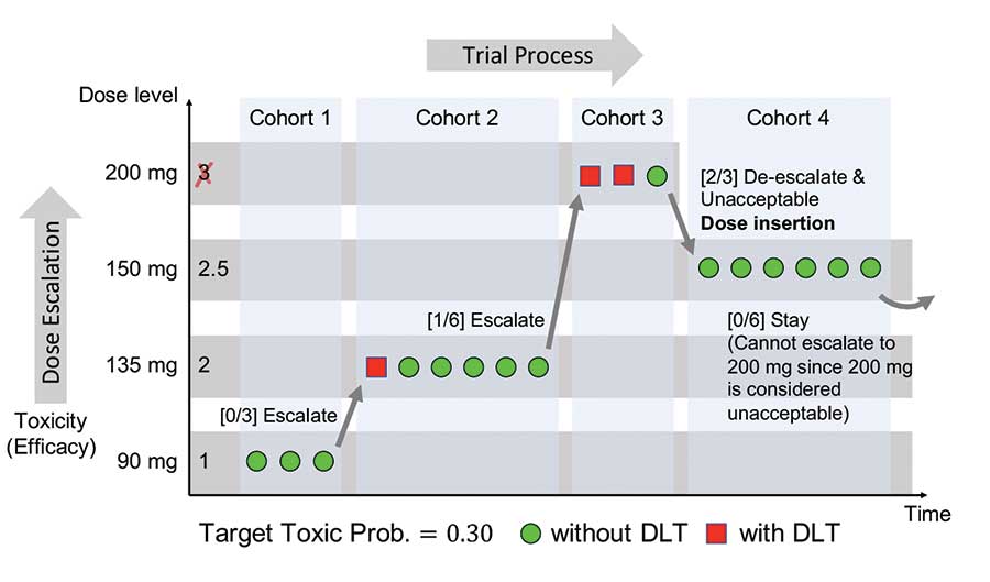
Figure 1. An illustration of the dose-finding study of dalotuzumab + MK-2206.
The i3+3 design. Even though the mTPI design has greatly simplified trial conduct, there is still room for further simplification, which is manifested in the cumulative cohort design (CCD) and later the Bayesian optimal interval (BOIN) design. Both designs use a point estimate, θ̃d = nd / (nd + md), to conduct statistical inference. Under a model-based framework, both designs view the point estimate θ̃d as the maximum likelihood estimator (MLE) or the posterior mode under a Beta(1, 1) prior for θd.
However, it is also true that θ̃d is simply the observed toxicity rate at dose level d, free from any statistical model. Motivated by this observation, the i3+3 design (Liu, et al. 2019.) was proposed as a design that abandons any models and returns to rule-based inference, but with smarter rules. This advancement completes the spiral evolution (Figure 2(a)) of the development of Phase I trial designs in the past three decades, shown as:
Rules → Complex Models → Simplified Models → Smart Rules.
In other words, statistical modeling seems unnecessary for dose-finding designs to generate desirable frequentist’s operating characteristics. This has been shown by the simulation results in the i3+3 design, along with its dose-assignment decision table in comparison with the aforementioned model-based designs.
Specifically, Figure 2(b) shows that the i3+3 design possesses almost identical decision tables as the mTPI and mTPI-2 designs, rendering highly similar operating characteristics.
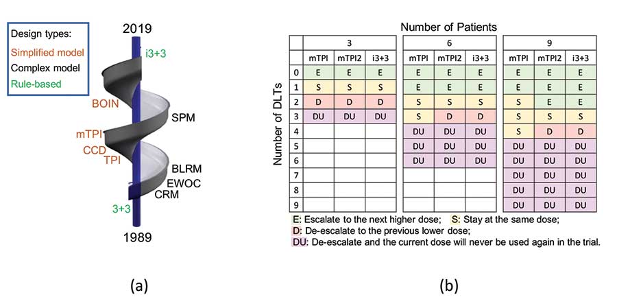
Figure 2: (a) Spiral evolution of dose-finding designs (1989—2019). (b) Decision tables of the mTPI, mTPI-2 and i3+3 designs with target rate θT = 0.3 (ε1 = ε2 = 0.05, and a dose is considered unacceptable (DU) when Pr(θd > θT|data) > 0.95).
Use of Historical Data
Many clinical trials involve the comparison of a new treatment to a control arm, e.g., the standard of care. Historical data are often available for the control arm, which can be obtained from previous clinical studies or routinely collected healthcare data such as electronic health records. With historical data providing information about the control arm, more resources can be devoted to the new treatment. As a result, it is usually desirable to incorporate historical data in the design and analysis of the current trial.
There are two main Bayesian methods for incorporating historical data. The first is to construct an informative prior for the parameters in the current control arm based on the historical data. The second is to model the current control arm parameters and the historical control parameters as random samples from a common population distribution, i.e., hierarchical modeling.
Informative Prior. To illustrate the construction of an informative prior, recycle the notation θ and let it denote the parameter of interest of the control arm of the current study. For example, for trials with a binary endpoint, θ is the control response rate; for trials with a continuous endpoint, θ is the mean response of the control arm. Denote the observed data and likelihood function for the current control arm by y and L(θ|y), respectively. Next, denote the historical data by yH, and let π0(θ) denote the initial prior distribution for θ before the historical data are observed, e.g., a non-informative prior. The power prior approach is a commonly used method to construct an informative prior for θ.
Specifically, the power prior distribution for θ is defined as:
πPP(θ | yH,α) ∝ π0(θ) ∙ L(θ | yH)α,
where α∈[0, 1] controls the weight of the historical data. When α = 1, πPP(∙) corresponds to the posterior distribution of θ from the previous study; when α = 0, πPP(∙) reduces to the initial prior and does not involve the historical data. In practice, the weight α may be pre-specified by the investigator or estimated from the observed data. The power prior can be generalized if multiple historical datasets are available.
As an example, consider a randomized controlled Phase II trial with the primary endpoint being the overall response rate (ORR). Suppose that in a historical study, 10 patients received the control treatment, among whom four patients had responses. Starting from a Beta(1, 1) prior on the control ORR before the historical study, the power α prior is Beta(1 + 4 ∙ α, 1 + 6 ∙ α), which can be used as an informative prior for the current control arm. Suppose further that we observe 6 responses out of 12 patients in the current control, the posterior of the control ORR is Beta(7 + 4 ∙ α, 7 + 6 ∙ α). Figure 3(a) shows this posterior density with different choices of α.
Hierarchical Models. The hierarchical modeling approach is another way to borrow historical information. Suppose, more generally, J historical studies are available (J can be 1). Let θHJ denote the corresponding parameter for historical study j. Assuming θ, θH1,…, θHJ are correlated and a priori exchangeable, they can be modeled as random samples from a common population distribution G. For example, if θ is the mean response, one can model
θ, θH1,…, θHJ | μ, τ ∼ N(μ, τ2).
In effect, the estimated mean response for the current control arm is shrunk toward the overall mean μ across all studies. The standard deviation parameter τ characterizes the degree of shrinkage. A smaller τ indicates more similarity across studies and more borrowing, while a larger τ represents more heterogeneity across studies and less borrowing. By placing priors on μ and τ, these parameters can be estimated from the data. When the number of historical studies is small (e.g., J = 1), the estimation of τ can be sensitive to the prior specification.
Consider again the randomized controlled Phase II trial example. By modeling the current and historical control response rates as random samples from a common population distribution, the estimated response rate for the current control arm is down-shifted toward the overall mean. See Figure 3(b).
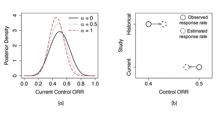
Figure 3. Illustrations of (a) the power prior approach and (b) the hierarchical modeling approach for incorporating historical data. Panel (a) shows the resulting posterior distribution of the control ORR with different choices of the power prior distribution. Panel (b) demonstrates the “shrinkage toward the overall mean” effect under hierarchical modeling.
Subgroup Analysis and Enrichment Designs
Subgroup analysis is about inferring patient subpopulations with distinct treatment effects and typically focuses on identifying a subgroup that benefits more from the investigational treatment compared to the overall population. For example, it may be of interest to explore whether a new treatment is effective in a particular subgroup of patients, given that the treatment is shown to be ineffective in the overall population through a randomized controlled trial.
Subgroup analysis can be naturally cast as a regression problem. Let Y, T, and X = (X1,…, XK) denote a patient’s response, treatment assignment, and baseline covariates, respectively. The subgroup effect can be characterized by the interaction between T and X. With a continuous response variable, the regression model has the form:
E(Y) = θ + Tγ + XTβ + TXTη
The regression coefficient η reflects subgroup effects, and testing “whether there is a subgroup effect” is equivalent to testing “whether η = 0“. Alternatively, tree-based methods can be used to better capture complex and nonlinear relationships among predictors. Consider a binary tree 𝒯 with each internal node corresponding to a splitting rule of a covariate Xk. Then, the terminal nodes of 𝒯 define a partition of the covariate space into subspaces, denoted by {𝓍1,…,𝓍M}. With a continuous response variable, the tree model may be constructed as:
E(Y|𝒯) = Σm=1 [βm ∙ 1(X ∈ 𝓍m) + ηm ∙ T ∙ 1(X∈ 𝓍m)].
Here, ηm represents the treatment effect within subspace 𝓍m (subgroup m), and the difference in ηm reflects subgroup effects. The tree 𝒯 itself is unknown and needs to be pre-specified or estimated from the data. Inference of the model parameters can be carried out under the Bayesian framework.
The challenges of subgroup analysis include the issue of multiple testing, lack of power, and the possibility of data dredging. Bayesian methods may partially address the issue of multiplicity through the use of priors. For example, in the regression model, spike and slab priors can be placed on η to shrink the interaction terms toward zero.
Similarly, in the tree model, subgroup-specific treatment effects ηm‘s can be shrunk toward a common value. It is also possible to simultaneously consider several competing models and use Bayesian model selection to pick a winning model. Priors can be constructed to favor parsimonious models.
Another type of method casts subgroup analysis as a decision problem consisting of two components: (1) inference for differential treatment effects and (2) an action of reporting subgroups. For the former, one can use flexible models to capture the relationship among Y, T, and X, e.g., E(Y|θ) = ⨍(T, X, θ), where ⨍ is a Bayesian additive regression tree model, and θ denotes additional parameters. For the latter, one can introduce a utility function u(S, θ) for the action of reporting a certain subgroup S, which usually has a preference for a large effect size, a large subgroup size, and a parsimonious description of the subgroup.
The optimal decision can be based on maximizing the posterior expectation of the utility function.
Subgroup analysis can be carried out to inform the design and decision-making of clinical trials. Subgroup-driven drug development usually consists of an exploratory trial and a confirmatory trial. The exploratory trial enrolls patients from a broad population with the goal of finding promising subgroups, and the confirmatory trial aims to establish health benefits with rigorous control of statistical error in the identified subgroups.
These two trials may be conducted seamlessly by adaptively learning the patient subgroups and restricting the inclusion criteria with the accumulation of data. The exploratory trial may also use response-adaptive randomization with a preference to allocate patients to the treatment arms from which they may be more likely to benefit.
Master Protocols
Conventionally, cancers are categorized based on the anatomic location of the primary tumor (e.g., breast, lung), and clinical trials in oncology are conducted to evaluate a single treatment in a certain cancer type. With recent advances in genomics, molecular engineering, and immunology, the paradigm of cancer treatment is shifting from “one size fits all” (e.g., cytotoxic chemotherapy) to targeted and precision therapies that aim to correct specific molecular or immune aberrations.
On one hand, a molecular or immune aberration can occur in a proportion of patients with different cancer types or subtypes of the same heterogeneous cancer.
On the other hand, a cancer (sub)type may harbor different aberrations that may be targeted by various therapeutics. Therefore, there have been increasing interest and successes in conducting clinical trials that test multiple treatments and/or multiple cancer (sub)types in parallel under a single protocol. Such trials are referred to as master protocols. See Table 1 for three examples.
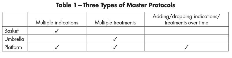
Table 1—Three Types of Master Protocols
Basket trials. Basket trials are a type of master protocol that consider a single treatment in multiple cancer (sub)types. Each group of patients with the same cancer (sub)type is then referred to as a basket. A recent successful case is the study of larotrectinib in different NTRK fusion-positive tumor types (see Figure 4(a)).
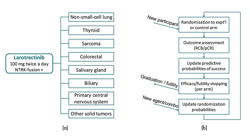
Figure 4. Illustrations of (a) the basket trial of larotrectinib in different NTRK fusion-positive tumor types and (b) the I-SPY 2 platform trial for breast cancer.
In a basket trial, the substudies are typically conducted in a single-arm fashion without concurrent controls. A popular choice of primary endpoint for exploratory cancer studies is the objective response rate (ORR), which can be observed relatively soon after treatment. In particular, the “objective response” consists of the partial response and complete response based on how much the tumor shrinks after treatment. The ORR in each substudy of a basket trial is compared with a historical control rate, and substudies with promising responses would warrant further investigation or conditional marketing approval. Since the same drug is tested, it is commonly assumed that the treatment effect of the drug in a certain basket can provide information about the treatment effects in other baskets.
Bayesian hierarchical modeling methods can be applied to borrow strength across different baskets and can often lead to improvements over stratified analyses in terms of estimation accuracy. Consider a trial with J baskets. Let θj and θ0j denote the treatment and historical control response rates in basket j, respectively. Further, let γj = log[θj / (1 − θj )] − log[θ0j / (1 − θ0j)] be the log-odds of the response rate in basket j after adjusted for the historical control rate. One can model:
γj ,…, γJ | μ, τ ∼ N(μ, τ2)
This model specification shrinks the adjusted response rates in different baskets toward a common value thus borrows strength across baskets. More complex and powerful models may replace N(μ, τ2) with a finite or infinite mixture distribution to induce a cluster-like structure.
Basket trials are usually planned with a pre-specified number of interim analyses. At each interim analysis, one can stop accrual for basket j early if Pr(θj > θ0j | data) < pF, where pF is a pre-specified futility stopping threshold, e.g., 0.05. After the trial completes, the rule for declaring efficacy in basket j can be based on Pr(θj > θ0j | data) > pE, where pE is a prespecified probability threshold for efficacy, e.g., 0.95.
A new application of basket trials is in multiple expansion cohort trials that proceed a dose-finding trial. (See FDA draft guidance in Further Reading.) In these types of trials, multiple doses of a drug may be expanded in multiple indications and an efficient statistical design that borrows strength across doses and indications is desirable. The same type of hierarchical models as described above can be considered.
Umbrella trials. These consider multiple treatments in a single cancer (sub)type and typically include a common control arm. More generally, platform trials may involve both multiple treatments and multiple cancer (sub)types and also include a notion of a perpetual process with treatment arms being added or dropped over time.
The BATTLE trial, as an umbrella trial, highlights the potential of combining different targeted treatments for a single cancer type: lung cancer. The I-SPY 2 trial (Figure 4(b)) is a prominent example of a platform trial, which evaluates multiple neoadjuvant treatments for high-risk breast cancer. Since these trials are concerned with multiple treatments in a heterogeneous patient population, methods for subgroup analysis also apply to the design and analysis of these trials.
For example, platform trials usually use response-adaptive randomization, so that better-performing treatments within a specific molecular signature would be preferentially assigned within that signature and will progress through the trial more rapidly.
To be specific, suppose a new patient with molecular signature x̃ is eligible for enrollment, and let q̃t denote the probability of response for this patient under treatment t, t∈{1,…,T}. Then, the probability of assigning the patient to treatment t can be proportional to Pr(q̃t > q̃t’ for all t’ ≠ t | x̃, data)α, where α∈[0, 1] is a pre-specified tuning parameter. At each interim analysis, each treatment’s posterior predictive probability of success in a Phase III confirmatory trial is calculated for each molecular signature.
A treatment arm would be dropped early (or be graduated), if this probability is low for all signatures (or is sufficiently high for some signatures) (see Figure 4(b)).
Other Methods and Future Directions
Several methods offer value for future efforts.
Seamless designs. Seamless designs allow two or more trials in different phases to be conducted within the same study. For example, Phase I/II seamless designs allow a Phase I dose-finding trial and a Phase II trial to be included in a single protocol, while Phase II/III designs combine Phase II and Phase III trials. In either type of seamless trial, an interim go/no-go decision evaluates whether the trial can transition from the earlier phase to the later phase. In the case of Phase I/II seamless design, such decisions graduate promising doses from Phase I to Phase II for further evaluation. For Phase II/III designs, the decisions determine whether a Phase II arm can be graduated or dropped and whether a Phase III trial is justified.
Future trial designs. It is an exciting era to be a trialist, due to the explosive innovation in the development of novel trial designs. Novel treatments based on molecular and immune markers and novel platform trial designs open new doors for Bayesian modeling and philosophy. In the future, trials are expected to become more adaptive, embracing modern computing power and adaptive decision-making.
For example, through complete blinding to sponsors of the entire trial process, it would be possible to conduct a trial that allows sequential interim analyses in which a trial can be stopped based on efficacy or futility posterior inference without adjusting for the frequentist Type I error rate inflation. Complete blinding is needed to reduce potential bias if the trial is not stopped during interim analyses.
On the other hand, future Bayesian designs and methods could incorporate repeated trials into multiplicity adjustment. This will help reduce the approval of potentially ineffective drugs that have failed in multiple prior trials but with positive results in a new confirmatory trial (e.g., the recent Alzheimer’s disease trials). In these settings, Bayesian designs could help enforce multiplicity control and limit the probability of making a wrong approval due to chance.
Impact of COVID-19. Coronavirus disease 2019 (COVID-19) is an ongoing pandemic affecting more than 200 countries and regions. The outbreak of COVID-19 can have an impact on oncology clinical trials in many aspects. For example, trial participants may be infected with, receive treatment for, or die from, COVID-19. Those who are not infected with COVID-19 may experience treatment discontinuations or interruptions due to the possibility of being exposed to infection, travel restrictions, or prioritization of COVID-19 patients. These issues are likely to impair the validity of the trial, so they require careful consideration by the trial conductor.
Methods for observational data and missing data, such as inverse probability weighting, can be useful for mitigating these issues. Guidance in the new ICH E9(R1) could be helpful to alleviate some issues from the frequentist point of view. However, it is a great opportunity to revisit Bayesian adaptive designs that use accumulated data and posterior probabilities for interim and final decision making for clinical trials.
In particular, Bayesian methods are ideal for “unplanned” interim looks, borrowing prior information, and calibrated posterior inference based on skeptical priors, which could potentially bridge the needs to use as much fragmented information from COVID-era trials and the desire to maintain statistical rigor, whether Bayesian or frequentist.
One central issue is the integrity of statistical inference in maintaining the Type I error rate. Type I error refers to a false-positive decision that rejects the null hypothesis, which typically leads to decisions that expose the drug to larger patient populations (e.g., market approval). These decisions may cause severe and costly public health and economic setbacks for society and drug developers. Due to random error and sampling noise in the trial data, statistical inference is always associated with the risk of Type I errors.
For example, whenever a null hypothesis in a clinical trial is rejected, e.g., a new drug is approved for public use, such approval is associated with a (ideally small) error probability. That is, the approval could be false. The probability of making a false rejection is unknown, but under the Bayesian framework, it can be estimated as the posterior probability of the null hypothesis, given the observed data. It is only possible to commit a Type I error when the null is rejected. If the null is not rejected, there is no Type I error and the Type I error rate is zero.
Based on such logic, a Type I error can only occur in a trial with multiple interim analyses and sequential decision points, if a positive decision, i.e., rejection of the null hypothesis, is made during an interim analysis. Otherwise, it is impossible to make a Type I error for that trial and that decision.
Conversely, once the rejection of the null hypothesis is made, the trial is usually stopped and no more decisions will be made. In this way, a Bayesian design with multiple interim analyses does not inflate the probability of making a false-positive decision or committing the Type I error. This is in contrast to the Type I error rate defined based on classical frequentist theory, which measures the frequency of false rejections in multiple hypothetical trials in which the treatment effect is assumed to follow the null hypothesis.
In summary, Bayesian interim analyses can be conducted “on demand” based on thresholding the posterior probability of the drug being effective without inflating the probability of making a wrong positive decision. This feature is crucial in helping resolve some challenges for COVID-era trials, in which unplanned interim analyses may be needed due to the pandemic.
Challenges in Bayesian Methods
While Bayesian methods are appealing in the design and analysis of clinical trials, they have their own caveats.
First, the choice of the prior distribution has an impact on posterior inference. Prior elicitation requires subject-matter expertise and good understanding of the probability model. If the prior is not well-constructed, posterior inference may be inefficient. Different investigators might provide different priors that lead to different posterior inference, and thus sensitivity analysis is recommended to examine whether the conclusion would substantially differ under various prior specifications. This increases the burden of using Bayesian methods in clinical trials.
Second, Bayesian methods do not necessarily have desirable frequentist properties; i.e., operating characteristics over possible repetitions of the same experiment. Usually, massive computer simulations are required to understand the frequentist properties of a Bayesian method, and calibration of the Bayesian method (e.g., calibration of the prior and probability threshold for decision-making) is needed to achieve desirable frequentist performance. When frequentist properties are strictly enforced, such as in confirmatory clinical trials, Bayesian methods are usually considered as supportive, although there has been fierce debate recently over whether frequentist properties (e.g., p-values) are the best criteria for decision-making.
Lastly, the posterior distribution for the parameter of interest does not have a closed-form expression in many situations, and computationally intensive Monte Carlo methods are necessary for inference.
Further Reading
Food and Drug Administration. 2018. Expansion Cohorts: Use in First-In-Human Clinical Trials to Expedite Development of Oncology Drugs and Biologics Guidance for Industry.
Food and Drug Administration. 2018. Master Protocols: Efficient Clinical Trial Design Strategies to Expedite Development of Oncology Drugs and Biologics.
Food and Drug Administration. 2010. Guidance for the Use of Bayesian Statistics in Medical Device Clinical Trials.
Nugent, C., Guo, W., Müller, P., and Ji, Y. 2019. Bayesian Approaches to Subgroup Analysis and Related Adaptive Clinical Trial Designs. JCO Precision Oncology 3, 1–9.
Viele, K., Berry, S., Neuenschwander, B., Amzal, B., Chen, F., et al. 2014. Use of Historical Control Data for Assessing Treatment Effects in Clinical Trials. Pharmaceutical Statistics 13(1), 41–54.
About the Authors
Tianjian Zhou is a postdoctoral scholar in the Department of Public Health Sciences at the University of Chicago. His research interests include clinical trial designs, statistical genomics, missing data, and infectious diseases. He earned his PhD in statistics from the University of Texas at Austin and received the Savage Award (honorable mention) for outstanding doctoral dissertations in Bayesian econometrics and statistics. He joined the Department of Statistics at Colorado State University as an assistant professor in fall 2020.
Yuan Ji is a professor of biostatistics at the University of Chicago and an NIH-funded PI focusing on innovative computational and statistical methods for translational cancer research. Ji is the author of more than 140 publications in peer-reviewed medical and statistical journals, conference papers, book chapters, and abstracts. He is the inventor of many innovative Bayesian adaptive designs, such as the mTPI and i3+3 designs, which have been widely applied in dose-finding clinical trials worldwide, including trials published in Lancet Oncology, JAMA Oncology, and JCO. He led a publication in Nature Methods and invention of a tool called TCGA-Assembler, which has been downloaded more than 10,000 times worldwide. He is also a co-founder of Laiya Consulting, Inc., which focuses on innovative and adaptive designs for clinical trials in new drug development, including the development of a novel early-phase statistical platform allowing seamless and efficient clinical trials with master protocols. He is an elected fellow of the American Statistical Association.


