
Challenging Nostalgia and Performance Metrics in Baseball

Introduction
It is easy to be blown away by the accomplishments of great old-time baseball players when you look at their raw or advanced baseball statistics. These players produced mind-boggling numbers. For example, see Babe Ruth’s batting average and pitching numbers, Ty Cobb’s 1911 season, Walter Johnson’s 1913 season, Tris Speaker’s 1916 season, Rogers Hornsby’s 1925 season, and Lou Gehrig’s 1931 season. The statistical feats achieved by these players (and others) far surpass the statistics that recent and current players produce.
At first glance, it seems that players from the old eras were vastly superior to the players in more modern eras, but is this true? This article investigates whether baseball players from earlier eras of professional baseball are over-represented among the game’s all-time greatest players according to popular opinion, performance metrics, and expert opinion.
Baseball players from “earlier eras” are defined as those who started their Major League Baseball (MLB) careers in the 1950 season or before because it coincides with the decennial U.S. Census and is close to 1947, the year in which baseball became integrated.
This article does not compare baseball players by their statistical accomplishments. Such measures exhibit era biases that are confounded with actual performance. Consider the single-season home run record as an example. Before Babe Ruth, the single season home run record was 27 by Ned Williamson in 1884. Babe Ruth broke this record in 1919 when he hit 29 home runs. He subsequently destroyed his own record in the following 1920 season when he hit 54 home runs. The runner-up in 1920 finished the season with a grand total of 15 home runs.
At that point, home run hitting was not an integral part of a batter’s approach. This has changed. Now, we often see multiple batters reach at least 30–40 home runs within one season and a 50 home run season is not a rare occurrence. In the 1920s, Babe Ruth stood head and shoulders above his peers due to a combination of his innate talent and circumstance. His approach was quickly emulated and became widely adopted. However, Ruth’s accomplishments as a home run hitter would not stand out nearly as much if he played today and put up similar home run totals.
The example of home runs hit by Babe Ruth and the impact they had relative to his peers represents a case where adjustment toward a peer-derived baseline fails across eras. No one reasonably expects 1920 Babe Ruth to hit more than three times the number of home runs hit by the second-best home run hitter if the 1920 version of Babe Ruth played today. This is far from an isolated case.
Several statistical approaches are currently used to compare baseball players across eras. These include wins above replacement as calculated by baseball reference (bWAR), wins above replacement as calculated by fangraphs (fWAR), adjusted OPS+, adjusted ERA+, era-adjusted detrending (Petersen, et al. 2011), computing normal scores as in Jim Albert’s work on a Baseball Statistics Course in the Journal of Statistics Education, and era-bridging (Berry, et al. 1999). A number of these are touted to be season-adjusted and the remainder are widely understood to have the same effect.
In one way or another, all of these statistical approaches compare the accomplishments of players in one season to a baseline that is computed from statistical data in that same season. This method of player comparison ignores talent discrepancies across seasons as noted by Stephen J. Gould in numerous lectures and papers. Currently, there is no definitive quantitative or qualitative basis for comparing these baselines, which are used to form intra-season player comparisons, across seasons. These methods therefore fail to compare players properly across eras of baseball despite the claim that they are season-adjusted.
Worse still, these approaches exhibit a favorable bias toward baseball players who played in earlier seasons (Schmidt and Berri. 2005). This bias can be explored from two separate theoretical perspectives underlying how baseball players from different eras would actually compete against each other.
The first perspective is that players would teleport across eras to compete against each other. From this perspective, the players from earlier eras are at a competitive disadvantage because, on average, baseball players have gotten better as time has progressed. Specifically, it is widely acknowledged that fastball velocity, pitch repertoire, training methods, and management strategies have all improved over time. Thus, the teleportation perspective is not of much interest.
The second perspective is that a player from one era could adapt naturally to the game conditions of another era if they grew up in that time. This line of thinking is challenging to current statistical methodology because adjustment to a peer-derived baseline no longer makes sense. Even in light of these challenges with the second perspective, the players from earlier eras are over-represented among baseball’s all time greats. These findings can be justified by considering population dynamics, which have changed drastically over time.
Data
The MLB-eligible population is not well-defined. As a proxy, the MLB-eligible population can be defined as the decennial count of males aged 20–29 who are living in the United States and Canada. Baseball was segregated on racial grounds until 1947. As a result, African American and Hispanic American population counts in the U.S. and Canada are added to the data set starting in 1960, chosen because the integration of the MLB was slow, as noted in Armour’s work on the integration of baseball in the Society for American Baseball Research.
Players from Latin, Central, and South American countries and the Caribbean islands were also targets of discrimination. Data from these countries have been added to the MLB-eligible population starting in 1960: Aruba, the Bahamas, Colombia, Cuba, the Dominican Republic, Honduras, Jamaica, Mexico, Netherlands Antilles, Nicaragua, Panama, Peru, Puerto Rico, the United States Virgin Islands, and Venezuela.
In the mid- to late 1990s, the MLB and minors saw an influx of Asian baseball players from Japan, South Korea, Taiwan, and the Philippines. The populations of these countries have been added to the MLB-eligible population starting in 2000.
In 2010, the MLB established a national training center in Brazil, as noted in Loré’s work on the popularity of baseball in Brazil in the Culture Trip. Therefore, the Brazilian population of 20- to 24-year-old men is included in the MLB-eligible population starting in 2010. It can be estimated that the 2011–15 MLB-eligible population is half of the MLB-eligible population counted in the 2010 decennial censuses. This can be expected to underestimate the actual 2011–15 MLB-eligible population since a constant increase in the overall MLB-eligible population has been observed as time increases.
The MLB-eligible population is displayed in Table 1. The cumulative proportion means that at each era, the population of the previous eras is also included. As an example of how to interpret this dataset, consider the year 1950. There were 11.59 million males aged 20–29. The proportion of the historical MLB-eligible population that existed at or before 1950 is 0.178.
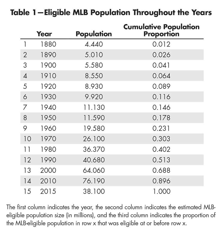
Table 1—Eligible MLB Population Throughout the Years
The Greats
To determine which are the all-time greatest players, four lists that reflect popular opinion, performance metrics, and expert opinion that purport to determine the greatest players can be consulted. The first list is compiled by Ranker, and is constructed entirely from popular opinion as determined by up and down votes. The second and third lists rank players by highest career WAR, as calculated by baseball reference and fangraphs, respectively. The fourth list is a ranking from ESPN and is based on expert opinion and statistics.
The rankings for all four lists are shown in Table 2. As an example of the information in Table 2, consider the greatest players of all time according to ESPN, displayed in the fourth column. Five players who started their careers before 1950 are in the top 10 all-time and 11 players who started their careers before 1950 are in the top 25 all time. When the MLB-eligible population is considered, it appears that the players from the earlier eras are over-represented in this particular list.
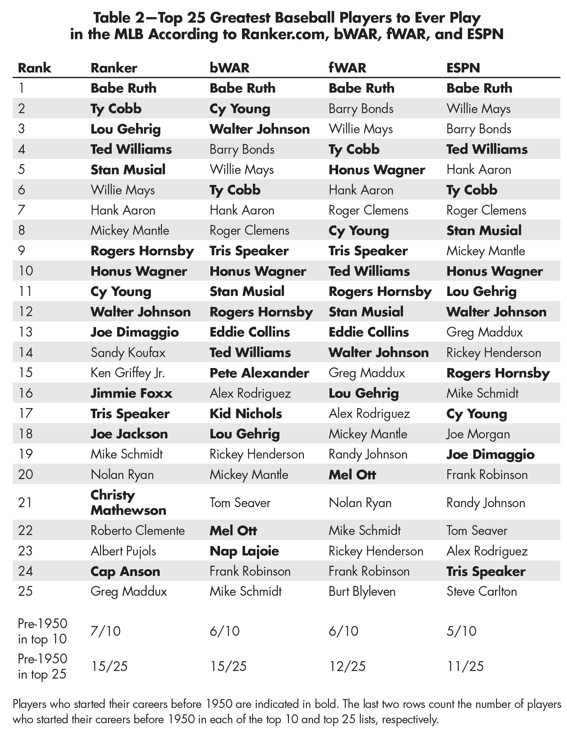
Table 2—Top 25 Greatest Baseball Players to Ever Play in the MLB According to Ranker.com, bWAR, fWAR, and ESPN
Statistical Evidence
Now there is evidence that the top 10 and top 25 lists displayed in Table 2 over-represent players who started their careers before 1950. Two assumptions are required for the validity of these calculations:
- First, innate talent is uniformly distributed over the MLB-eligible population over the different eras.
- Second, the outside competition to the MLB available by other sports leagues after 1950 is offset by the increased salary incentives received by MLB players.
With these assumptions in mind, the probability can be calculated that at least x people from each top 10 and top 25 list in Table 2 started their careers before 1950, using the proportion depicted in Table 1. Consider the bWAR list, for example. According to bWAR, six of the top 10 players started their careers before 1950. Table 1 shows that the proportion of the MLB-eligible population that played at or before 1950 was approximately 0.178. The probability that one would expect to observe six or more individuals in a top 10 list from that time period can be calculated based on this proportion using the binomial distribution. Performing the same type of extreme event calculation for each top 10 and top 25 list depicted in Table 2 provides the results in Table 3.
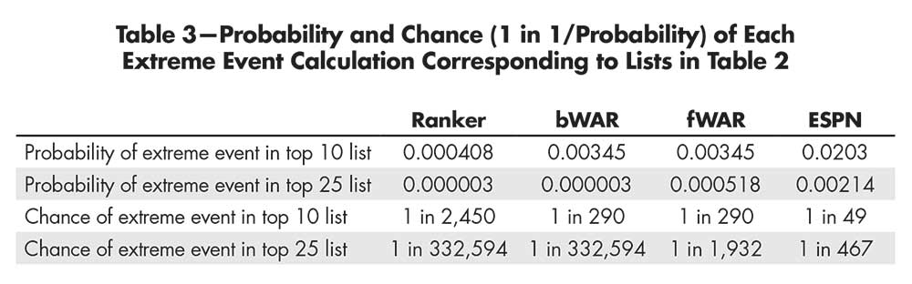
Table 3—Probability and Chance (1 in 1/Probability) of Each Extreme Event Calculation Corresponding to Lists in Table 2
As an example of how to interpret the results of Table 3, continue with bWAR’s top 10 list. Table 3 shows that the probability of observing six or more players who started their careers at or before 1950 of the top 10 all-time players, based on population dynamics, is about 0.00345 (a chance of 1 in 290). The same interpretation applies to the remainder of Table 3. The results in Table 3 present overwhelming evidence that players who started their careers before 1950 are overrepresented in top 10 and top 25 lists from the perspectives of fans, analytic assessment of performance, and experts’ rankings.
Assumptions and Sensitivity Analysis
The results in Table 3 are valid under the two assumptions above. The first of these assumptions specifies that innate talent is evenly dispersed across eras. It is not fully believable that the first assumption holds, because the distribution of innate talent has improved over time as the MLB-eligible population has expanded, as noted by Gould, Christina Kahrl at ESPN, and in Martin B. Schmidt and David J. Berri’s work on concentration of baseball talent in the Journal of Sports Economics. This suggests that the probabilities displayed in Table 3 are conservative.
With respect to the second assumption, the National Basketball Association (NBA) and National Football League (NFL) started in 1946 and 1920, respectively, with both sports greatly rising in popularity since the inception of their respective professional leagues. Soccer and hockey have also risen in popularity in the United States.
That being said, it is widely known that MLB salaries have increased substantially. For example, the 1967 census lists the median U.S. household income as $7,200. The minimum MLB salary at that time was $6,000, as noted by Los Angeles Times sports writer Bill Shaiken in a piece titled “A look at how Major League Baseball salaries have grown by more than 20,000% the last 50 years.”
In short, baseball players made far less than they do today relative to the general U.S. population, and it is unlikely that one could consider playing professional baseball to be a lucrative career in the earlier eras. These figures offer evidence that while other professional leagues may have drawn from the MLB-eligible talent pool, salary incentives have led to an increase in the overall quality of MLB players.
Although this theory cannot be confirmed with absolute certainty, the second assumption suffers modest violations at worst. To account for this possibility, applying a sensitivity analysis to the findings in Table 3 can be considered. The decennial populations displayed in Table 1 can be weighted to reflect the overall interest that the U.S. population has had in baseball over time, irrespective of salary increases based on Gallup polling data.
The four weighting regimes being considered are shown in Table 4 below. These regimes serve as proxies for the proportion of the MLB-eligible population thought to strive toward a career in professional baseball. In an effort to be conservative, greater weight have deliberately been placed on the time periods before 1940 for each weighting regime because no polling data are available. The MLB-eligible population before 1940 is not expected to be as high as the weighting regimes suggest because of relatively modest baseball attendance figures in early eras of baseball, non-existence of the radio prior to 1920, the dead-ball era, and low compensation.
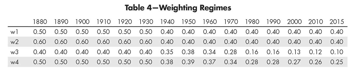
Table 4—Weighting Regimes
David W. Moore and Joseph Carroll’s Gallup article, “Baseball Fan Numbers Steady, But Decline May Be Pending,” shows that interest in baseball has remained steady since 1937, at approximately 40%. Consistent with this benchmark, the first and second weighting regimes (w1 and w2) conservatively place 0.50 and 0.60 weights, respectively, on fan interest before 1940. The third weighting regime (w3), constructed from the Gallup polling data in Figure 1, reflects the proportion of the U.S. population who listed baseball as their favorite sport.
The appropriateness of this regime is intuitively questionable, because some people play baseball even if it is not their favorite sport and the weight placed on pre-1940 years is very high.
The fourth weighting regime (w4) is the average of w2 and w3.
These weights are from survey data from the U.S. because similar data are not available from other countries. These same weights have been applied to all of the other countries, even though interest in baseball in these other countries is thought to either be on par with or much greater than in the U.S. Therefore, the weighting regimes address, and in fact, overcompensate for any potential shortcomings of no weighting.
Table 5 shows the effect of these weighting regimes as applied to the results in Table 3. The conclusions from weighting populations with respect to w1, w2, and w4 in Table 5 are largely consistent with those in Table 3, but the third weighting regime presents some conflicting conclusions: When weighting populations with respect to w3, popular opinion and bWAR still over-represent players who started their careers before 1950. However, the same is not so for fWAR and ESPN. The overall finding of this sensitivity analysis is that conservatively weighting populations with respect to fan interest in baseball yields the same conclusion as the analysis in Section 4: It is very unlikely that the pre-1950s time period could have produced so many historically great baseball players.
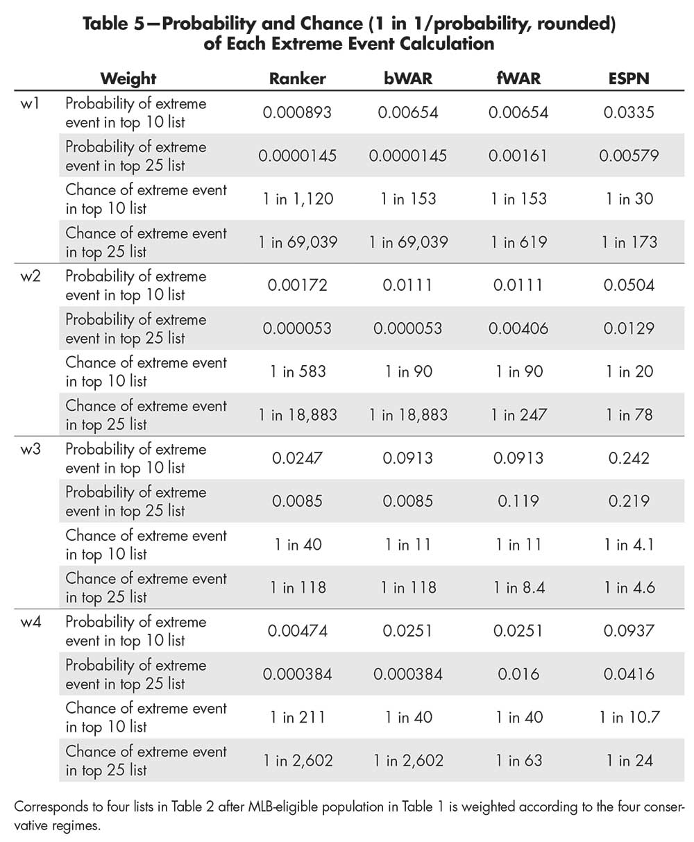
Table 5—Probability and Chance (1 in 1/probability, rounded) of Each Extreme Event Calculation
Methods Other than Your Peers
Several methods are used to compare players across eras by computing a baseline achievement threshold in one season and then comparing players to that baseline. These methods then rank players by how far they stood above their peers; the greatest players were better than their peers by the largest amount. This approach can exhibit major biases in player comparisons, as evidenced by career bWAR and fWAR. Adjusted OPS+ is a worse offender than bWAR or fWAR. Adjusted ERA+ is right in line with ESPN rankings.
PPS Detrending
The methodology of Petersen, et al. (2011) (PPS) detrends player statistics by normalizing achievements to seasonal averages, which PPS claim accounts for changes in relative player ability resulting from both exogenous and endogenous factors, such as talent dilution from expansion, equipment and training improvements, and performance-enhancing drug usage. However, PPS misunderstand the effect of talent dilution from expansion and ignore reality.
The talent pool was more diluted in the earlier eras of baseball than now because of a relatively small eligible population size and the exclusion of entire populations of people on racial grounds (see Table 6 for specifics). PPS’s position with respect to equipment and training improvements is likewise not without fault, because the same improvements are equally available to every competitor. Finally, PPS do not account for increases in salary compensation enjoyed by MLB players in modern eras, and their methodology fails to address segregation before 1947.
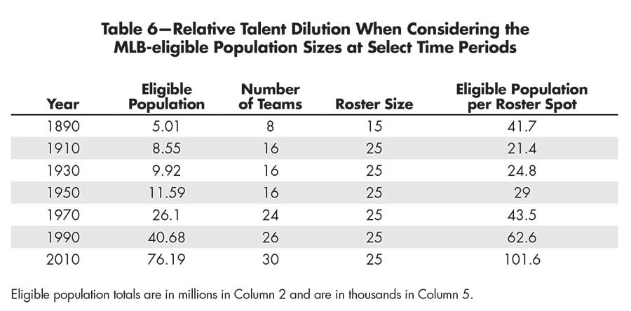
Table 6—Relative Talent Dilution When Considering the MLB-eligible Population Sizes at Select Time Periods
The mathematics of PPS detrending are also questionable in the context of comparing baseball players across eras. PPS note that the evolutionary nature of competition results in a non-stationary rate of success. They then detrend player statistics by normalizing achievements to seasonal averages as follows: Suppose a player hits 40 home runs in a given season and the league average prowess for home run hitting in that season is 10 home runs. If the historical average prowess for home run hitting is five home runs, then the player’s detrended home run count in that particular season is 40 × (5/10) = 20. In general, the detrending formula is Y × (historic prowess/league prowess) where Y is individual prowess for a particular player in a given season. PPS detrending can be seen as an inflationary metric of relative prowess and not a detrending metric.
Authoritative textbooks such as Introduction to Time Series and Forecasting, by Peter J. Brockwell and Richard A. Davis, advocated fundamentally different approaches for detrending. Table 2 in PPS displays the top 25 career detrended home run totals. It is clear that having higher prowess relative to peers—hitting more runs, in this case—is not indicative of a player’s prowess with respect to peers from fundamentally different eras.
Era-bridging
Berry, et al. (1999) claim that their era-bridging technique accounts for talent discrepancies across eras. However, they do not explicitly parameterize this in their hierarchical models. They state that “globalization has been less pronounced in the MLB (relative to other sports)…Baseball has remained fairly stable within the United States, where it has been an important part of the culture for more than a century.” This rationale ignores segregation, increases in the MLB-eligible population relative to available roster spots, and increases in the average overall talent of that population. Therefore, their methodology does not fully address the characteristics of a changing talent pool.
In Berry, et al. (Panel (c) of Figure 7), the model predicts that a .300 hitter in 1996 will have a lower than .300 average for several seasons from 1900–20. This conflicts with the well-established notion that the talent of baseball players has improved over time. Berry, et al. (Table 9) shows that six of the 10 best hitters by average started their careers before 1950 and 10 of the 25 best hitters by batting average started their careers before 1950. This paper was published in 1999, and the chances of these events can be recomputed where the MLB-eligible population ends at 1999. The chance of expecting to observe six or more individuals in a top 10 list who started their careers before 1950 is 1 in 38. The chance of expecting to observe 10 or more individuals in a top 25 list who started their careers before 1950 is 1 in 9.99.
These chances are not as extreme as those in Table 3, but they still correspond to events that are unlikely.
Conclusions
The MLB players from the early eras of baseball receive significant attention and praise as a result of their statistical achievements and their mythical lore. These players are collectively over-represented in rankings of the greatest players in the history of the MLB, and popular performance metrics such as WAR fail to compare players properly across eras. Superior statistical accomplishments achieved by players who started their careers before 1950 are a reflection of the inability to properly compare talent across eras. It is highly unlikely that athletes from such a scarcely populated era of available baseball talent could represent top 10 and top 25 lists so abundantly.
As a general discussion of greatness, the conclusions in this article have broader implications than just rankings of athletes. Who are the greatest actors and actresses, artists, musicians, scientists, revolutionaries, or leaders who have ever lived? Do our perceptions change when we focus beyond nostalgia? Do our perceptions change when we recognize and properly account for gender and racial discrimination that has existed throughout human history into the present day?
Further Reading
Berry, S.M., Reese, C.S., and Larkey, P.D. 1999. Bridging Different Eras in Sports. Journal of the American Statistical Association 94, 447, 661–676.
Petersen, A.M., Penner, O., and Stanley, H.E. 2011. Methods for detrending success metrics to account for inflationary and deflationary factors. European Physical Journal BM 79, 67–78.
Schmidt, M.B., and Berri, D.J. 2005. Concentration of Playing Talent: Evolution in Major League Baseball. Journal of Sports Economics 6, 412–419.
About the Author
Daniel Eck is an assistant professor of statistics at the University of Illinois Urbana-Champaign. Previously, he was a postdoctoral associate at Forrest Crawford’s lab in the Department of Biostatistics at Yale University. He obtained his PhD from the Department of Statistics at the University of Minnesota in 2017.


