
The Importance of Data Cleaning: Three Visualization Examples
An article in the New York Times, “For Big-Data Scientists, ‘Janitor Work’ Is Key Hurdle to Insights,” said that data scientists spend 50% to 80% of their work time on cleaning and organizing data, leaving little time for actual data analysis. Even worse, data scientists may have a difficult time explaining delays to their stakeholders, especially when emerging analysis reveals additional data issues that have to be resolved. Data scientists can use these examples to help non-technical collaborators appreciate the importance of data cleaning.
Data analysis tools are powerful in business, but businesses need data to be cleaned appropriately before they can produce valid outputs. Otherwise, the whole data pipeline becomes “garbage in, garbage out,” and the result would not be as useful as a business team expected. An article in a 2018 Harvard Business Review, “If Your Data Is Bad, Your Machine Learning Tools Are Useless,” also regarded poor data quality as the number-one enemy of machine learning.
Real data are never perfect because data errors are inevitable and may occur in creative and unexpected ways. For example, respondents may misunderstand questions, leading to incorrect responses; software used for data processing may substitute incorrect values when it cannot interpret a given value; even simple spelling mistakes can affect results.
Fortunately, many of these mistakes can be corrected using inferences made through analysis of other variables. Analysis of contradictory information in the same variable, across different variables, outliers, and duplicated records with inconsistent responses, may all be used to clean up data.
This article provides three examples of common data issues and explains how to identify and fix them quickly. Visualizations compare data quality before and after cleaning. These demonstrations make it easier for data scientists to justify their data processing time to stakeholders without using too much jargon.
The first example, “Missing Values Encoded as 99,” shows how missing data encoded as invalid values would affect a regression. The second example, “Dollars vs. Thousands of Dollars,” describes how an unreasonably small dollar amount can be due to respondents confusing “dollars” with “thousands of dollars.” The third example, “Invalid Dates in Records,” explains how invalid dates can be corrected by additional records for the same person.
These examples do not represent all possible methods of data cleaning, but adequate exploratory data analysis can uncover many data issues before any modeling is performed. In other words, identification of data problems is often supported by data explorations, not just by advanced statistical methods. (Note that all data used in this article are fictitious and for demonstration purposes only.)
Example 1: Missing Values Encoded as 99
Assume we have data on people’s years of education and annual incomes, and we would like to quantify the relationship between the two variables. However, when we plot the raw data in Figure 1, the regression line is severely distorted because some people have 99 years of education! It is unreasonable to have 99 years of education because most people do not even live that long, so such data points are most likely to be data errors. As a comparison baseline, people who completed high school typically have 12 years of education, and people with a college degree or equivalent would be counted as having 16 years of education.
In fact, the distorted regression line is due to missing values encoded as 99 in the variable “Years of Education.” In statistical software, a missing value is often replaced with a placeholder numeric value for consistency of record type. The placeholder numeric value is a number that is obviously unreasonable, so it is easy to tell that the actual value is missing. An alternative is to encode “-1” for missing values. This value is similarly unreasonable because a person cannot have fewer than 0 years of education.
Figure 1 shows that the missing values encoded as 99 severely distort the regression results, so the ordinary linear model does not fit well. Moreover, it is difficult to examine the details for people with 0 to 20 years of education because they are squeezed into the left side of the x-axis. Therefore, we should remove the 99s and run the regression on only the non-missing data in this case. In Figure 2, the model fits much better, and the positive association between years of education and annual income can easily be seen.
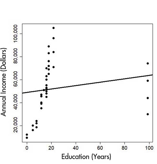
Figure 1. Before data cleaning.
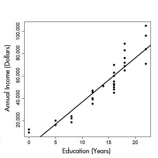
Figure 2. After data cleaning.
The reason for missing data must be explored because this step would inform the type of analyses/models required to address the issue. In this example, we removed missing data for years of education because we have no way to infer the underlying correct value. In other situations, it can be beneficial to make efforts to correct the raw data.
Example 2: Dollars vs. Thousands of Dollars
This example originated from the National Survey of Mortgage Originations at the Federal Housing Finance Agency. The agency mails quarterly surveys to collect information from borrowers or mortgagees to understand what borrowers think about when taking out loans. Then it publishes the aggregated results to assist other federal agencies in making mortgage policy decisions.
The survey data are not always accurate due to respondent errors. Thus, we need to understand the metadata—the information about the data set—to identify what can potentially go wrong. This example demonstrates the confusion of units: People may mistake “dollars” as “thousands of dollars.”
We do not have the actual data, so we generated fictitious data to reflect the issue. For instance, the original data may show that someone took out a mortgage for 1,400 dollars, which is an unusually small amount, so it is more likely that the respondent meant 1,400 thousands of dollars, or a mortgage of $1.4 million ($1,400,000).
Since the data contain both the mortgage amount and the property purchase price, we can perform error correction if only one of them is wrong. We can safely assume that the higher the property purchase price, the higher the mortgage amount. Figure 3 plots the original (fictitious) data for the relationship. One data point at the bottom right had a purchase price of $1.5 million, but a small mortgage of $1,400. As a result, the regression line has a poor fit due to the datapoint as an outlier.
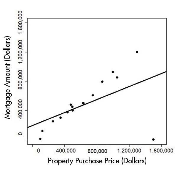
Figure 3. Original data.
After modifying the mortgage to $1.4 million, we can see in Figure 4 that the regression fits much better.
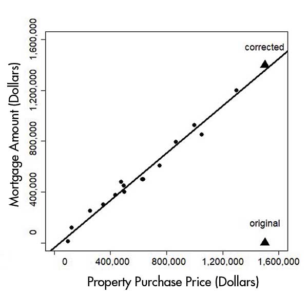
Figure 4. Corrected data.
This example provides insights into potential errors of a large magnitude, since the number of dollars and thousands of dollars differ greatly. However, when both mortgage amount and property purchase price are potentially mistaken in the magnitude of dollars, it is more difficult to detect the error. In some cases, the dollar amounts can be actually correct.
Assume that a record shows a person took out a $2,500 loan to buy a $3,000 single-family house in 2010. A house for $3,000 is impossible in the current housing market, but this could have been possible in the early 20th century, before house prices started to skyrocket. The underlying mistake may be the record date: It turns out that the mortgage was issued in 1940, rather than 2010.
Example 3: Invalid Dates in Records
In addition to numerical value errors, invalid dates are also common in data. It is necessary to incorporate range checks in the data exploration step, so variables with a specific range, such as dates, can be easily validated. For example, a person cannot be born later than today’s date, so the birth year 2048 is invalid. If the record shows that the person was born on July 40, that is also an invalid date. Thus, we would like to demonstrate a potential remedy by borrowing information from additional records for the same person.
We used the data set RLdata10000 from the R package RecordLinkage. The data contain 10,000 artificial person records, which include 9,000 distinct records and 1,000 duplicates with at least one error. Each person record contains the person’s first name, last name, birth year, birth month, and birth day. The identity.RLdata10000 data set in the same R package shows which records in RLdata10000 belong to the same person, so we already know the ground truth and do not have to relink the record ourselves.
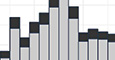
Some of the duplicate records contain invalid dates. Attempting to plot the birth years results in an extremely skewed histogram in Figure 5, which is ugly and uninformative. A birth year 9185 at the rightmost side of the graph squeezes all the other birth years of less than 2500 into a single column. The birth year 9185 is obviously invalid, so we need to dive deeper into the RLdata10000 to uncover and correct additional invalid dates.
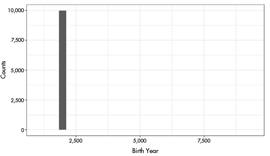
Figure 5. Birth year histogram of raw RLdata10000 records.
To amend the invalid dates, we compare the records of the same person. Table 1 shows part of the RLdata10000. The records of the same person are paired up. When two records belong to the same person, one record can be used to “correct” the other record’s invalid date of birth. This examples assumes that the record with a valid date of birth is accurate. We also assume that a valid birth year would fall between 1900 and 2019. In Table 2, the birth year 9185 is corrected to 1985, the birth month 13 is corrected to 11, and the birth day 72 is corrected to 22. After we made a change in a value, we also flagged the record as “corrected” in the appropriate column for future reference.
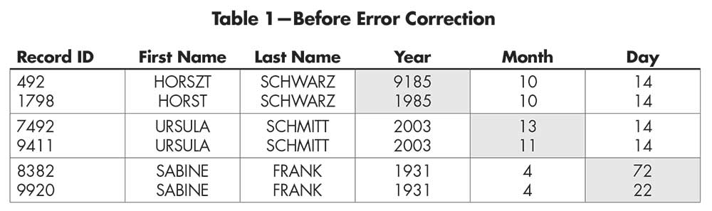
Table 1—Before Error Correction
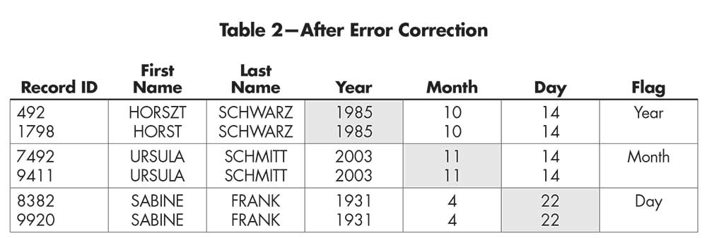
Table 2—After Error Correction
Finally, plotting the histogram of all valid birth years in RLdata10000 in Figure 6 looks much more informative. The histogram also indicates which records are distinct (i.e., non-duplicate) and which ones are duplicates. Identifying duplicate and/or erroneous records helps in data cleaning, so it is important to remove unwanted records early in the pipeline.
Although it is clear that errors can be fixed, error correction has its limitations. For instance, when both dates in a record pair are valid, external information is needed to verify which is correct. Moreover, errors in names are harder to identify and correct. In Table 1, “Horst” and “Horszt” would be considered two different people, but the two records belong to the same person. The “z” in the latter name is probably a typo.
One potential solution is to compare the records against a dictionary of first and last names. In the record pair, if only one record is a name in the dictionary, the other one can be corrected to the dictionary-defined name.
Advanced Statistical Methods
To further improve the data cleaning process, advanced statistical methods are needed for non-obvious errors that may still affect an analysis. For example, some respondents were confused by the rating scale in a questionnaire, resulting in flipped ratings: The score was assigned the opposite of the rating scale.
The 1–10 rating scale can mean at least two concepts:
- 1 = least important and 10 = extremely important
- 1 = low priority and 10 = high priority
When we adopt the second definition of a 1–10 rating scale, a respondent may give a 1 rating with the comment “This task is crucial and we should work on it as soon as possible.” The respondent meant 10 (high priority) but unwittingly reversed the rating scale.
If we visualize the percentages of each rating, the results would not be accurate. However, the rating error would not be detected if we simply plot the histogram of the rating. When additional information is available in the exploratory phase, though, such as text comments by the respondents, we may discover these issues in the data.
For a large number of responses, we need to create an automatic pipeline to analyze the text, estimate the underlying rating, and make the correction. A potential solution is to use the supervised latent Dirichlet allocation (sLDA) to predict the rating from the text comment.
Conclusion
Data cleaning is essential in preparing data for analysis, and it is important to handle potential data errors before presenting results. Comparing model results with and without the data errors allows presentation of graphical evidence to show that data cleaning is worth the time spent. Even though error correction is not always perfect, the process still improves the data quality.
It has been said that “A picture is worth a thousand words,” and this could not be more true in data visualization. By using graphs and tables, we visualized the importance of data cleaning, making it easier to understand for people without a technical background. This is expected to improve the communication between data scientists and stakeholders.
Acknowledgments
The author is grateful for the support of Microsoft, and gives special mention to her colleague Larissa Cox for feedback on the draft version. The author would also like to thank the anonymous reviewers for their helpful comments.
Further Reading
Chai, C.P. 2019. Text Mining in Survey Data. Survey Practice 12(1). doi: 10.29115/SP-2018-0035.
Federal Housing Finance Agency. n.d. National Mortgage Database Program.
Fisher, N.I. 2019. Supplementary Material to A Comprehensive Approach to Problems of Performance Measurement. Journal of the Royal Statistical Society: Series A (Statistics in Society) 182(3):755–803. doi: 10.1111/rssa.12424.
Lohr, S. 2014. For Big-Data Scientists, “Janitor Work” Is Key Hurdle to Insights. New York Times.
Martin, E. 2017. Here’s how much housing prices have skyrocketed over the last 50 years. CNBC.
Redman, T.C. 2018. If Your Data Is Bad, Your Machine Learning Tools Are Useless. Harvard Business Review.
About the Author
Christine P. Chai is a software engineer at Microsoft, but her work is similar to that of a data scientist. She analyzes retail data as part of a team to create actionable insights, such as estimating the store traffic from a local event to improve retail sales prediction. Before joining Microsoft, she completed a PhD in statistical science at Duke University in 2017 and worked in the federal government for a while.


