
Replicability, Reproducibility, and Multiplicity in Drug Development

Replication of research findings is fundamental to good scientific practice. The inability to replicate experimental results in subsequent experiments, either by independent investigators or by the original investigators themselves, could severely compromise the interpretability and credibility of the scientific claims. However, since John Ioannidis’s 2005 influential paper “Why most published research findings are false,” awareness is growing in the scientific community that the results of many research experiments are difficult or impossible to replicate. In the meantime, this discussion has reached the public mainstream, aptly coined as the “replication crisis,” with examples from virtually every scientific discipline.
Clarity on concepts
The replication crisis has long-standing roots, but a lack of clarity remains about fundamental concepts. For example, “replicability” and “reproducibility” are often used interchangeably, although scientists usually discuss the need to replicate an experiment, not to reproduce it.
While there is no universally agreed-upon definition of these terms, “reproducible research” seems to have a clear meaning in parts of the scientific community. Publications such as the Biometrical Journal and Biostatistics were early adopters of the idea that the ultimate product of academic research is a scientific paper supported by presentation of the full computational environment used to produce (and reproduce) the paper’s results (such as the code, data, etc.). Replicability, on the other hand, is commonly used to describe the ability to repeat results of an experiment by a subsequent experiment of the same (or, at least, a similar) design, executed by the same or different investigators.
What constitutes a successfully replicated experiment may not always be clear, though. It is unreasonable, if not even unrealistic, to expect that every detailed result from a scientific experiment can be replicated in a subsequent experiment. This is particularly true in areas such as psychology and medicine, where investigators are faced with highly variable observations. Even in an ideal world, we would expect to see some (more or less) random deviation in the results and conclusions in independent experiments. The validity of such conclusions can never be definitively proven, but the belief in their truth can be strengthened by achieving the same or similar results when independently replicating the experiment.
That means reasonable replicability criteria have to be specified in advance that allow investigators to claim a successful replication experiment. One such possible criterion could be that the estimate of the parameter of main interest in the replication experiment is covered by a two-sided 95% confidence interval derived from the first experiment. Interestingly, assuming that the two experiments have the same design (including the same sample size) and the estimates are approximately normal distributed with known variance, the probability for claiming a successful replication — even if the settings are identical — is about 83%. This is considerably less than the 95% one might expect, which is the confidence level for the true (unknown) parameter.
More generally, assuming that the size of the replication experiment is m times the size of the initial experiment, the probability Prep for a successful replication in the above sense, with respect to a two-sided 100(1 – α)% confidence interval for αε (0,1), is
![]()
where Φ denotes the cumulative distribution function of the standard normal distribution.
The reason for the reduced probability Prep < 1 – α is that both original and replication experiments bear some uncertainty about the true parameter value. This alone, however, cannot explain the seeming difficulty in replicating findings, with reported success rates as low as 40% in many scientific disciplines.
While many causes for the observed lack of replicability have been cited, failure to account for multiplicity is likely to be a culprit. This article uses “multiplicity” in a broader sense than traditionally linked with terms like “multiple comparison procedures” and “multiple testing.” Fishing for significance, data dredging, and selection bias (including publication bias due to non-reporting of negative results) are all facets of the same problem: that seemingly prominent results may occur more often than expected by chance alone. Failure to compensate for multiplicity can have important real world consequences and contribute to the replication crisis.
Pharmaceutical drug development is an area that is particularly prone to a lack of replicability. Research and development of a drug is an expensive and time-consuming process that may last more than 10 years and cost as much as $2.5 billion on average, with attrition rates of well over 50%. This process spans discovery in the laboratory, preclinical safety testing, first-in-human-studies of safety and tolerability (Phase I), dose-ranging studies to identify the best doses (Phase II), confirmatory testing of those doses to demonstrate safety and evidence of effectiveness (Phase III), and postapproval studies of other uses (Phase IV).
Against this background, John Tukey conceded in his 1977 paper “Some thoughts on clinical studies, especially problems of multiplicity” that “once multiple questions are to be asked, there will be pressures, some ethical in nature, to concentrate upon those questions for which the results appear most favorable.” As an illustration, consider the situation of conducting two independent clinical studies in sequence; call them Studies 1 and 2. Assume that Study 1 compares a new drug with placebo in four distinct patient populations (e.g., female and male patients for two age classes). At the end of Study 1, we select the “best” population (i.e., the one with the largest observed treatment effect, compared to placebo) for Study 2, with the objective to replicate and confirm the findings from Study 1.
Assume the same true treatment effect size and variability of the observations in the four populations and both studies. If we repeat Study 2 many times, the average observed effect size for the selected population in Study 2 will be considerably smaller than in Study 1. This lack of replicability is, of course, due to the “random high” bias in the estimate obtained by selecting the best population. That is, the expected value of the estimate of the best population is larger than that of a randomly selected population. The expected difference between these estimates (i.e., bias) depends on their distribution, but can be quantified independently of the distribution as follows.
Assume that there are k non-overlapping populations with a common (unknown) treatment effect size θ, where larger values indicate a better outcome. Denote by Li the (random) lower bound of a one-sided 100(1 – α)% confidence interval for θ based on the data of population i = 1, …, k. Assume for simplicity that the best population j is defined as the one with the largest lower bound, i.e., Lj = max {Li: i = 1, …, k}.
Selecting the best population according to confidence limits and not according to parameter estimates has its merits. For example, when investigating two populations of grossly unequal sizes, assume that the mean effect in the smaller population is slightly larger than the one in the larger population. The confidence limit for the smaller population is, then, far away from the mean and much smaller than the confidence limit for the larger population. Thus, we can be fairly sure that the true parameter value in the larger population is not small, but we cannot be sure about the effect size in the smaller population, so it is safer to declare the larger population as the “best.”
For this definition of the best population, the probability that the confidence interval with lower bound Lj covers the true value θ is 100(1 – α)k % regardless of the distribution of the estimate. For example, for k = 4 and 1 – α = 0.9, this probability is 65.6%. However, the probability that the observed sample mean of Study 2 is at least as large as Lj can be even smaller. For example, assuming equal sample sizes in all populations, asymptotic normality of the estimates and that the replication study has m = 4 times the number of patients from the same population in Study 1, this probability reduces to 62.4% for k = 4 and 1 – α = 0.9. Under these assumptions, the selection of the best by the largest estimate and by the largest confidence bound are equivalent.
In general, the probability for a successful replication under these above assumptions is
![]()
where the random variables Vi are jointly multivariate normal distributed with E(Vi) = 0, Var(Vi) = 1 + 1/m and Cov(Vh,Vi) = 1/m, h ≄ i. Note that Prep decreases for larger values of k but can be larger than (1 – α)k. For example,
Prep = 36.3% > 34.9% = 0.910 for k = m = 10 and 1 – α = 0.9.
These numerical examples illustrate the close link between replicability and multiplicity. Failure to account for multiplicity can lead to a lack of replicability, which in turn can have various untoward consequences. For example, when drug efficacy is involved, it may result in the approval of a drug as an improvement over existing drugs, when there is in fact no beneficial effect. On the other hand, when drug safety is involved, the new drug could appear to be worse for some side effect when it is actually not worse at all, preventing a beneficial drug from being approved. Multiple hypothesis testing is therefore becoming increasingly important, particularly in confirmatory Phase III clinical studies, since these studies form the basis for drug approval by regulatory agencies worldwide.
The following examples describe how multiplicity raises challenging problems that affect important decisions throughout drug development, and how different sources of multiplicity may require very different strategies for addressing those problems.
Graphical Test Procedures
Given the pressure under which drug development takes place, pharmaceutical companies and other trial sponsors want to learn as much as possible from every study, leading to increasingly extensive and complex clinical study objectives. These objectives could include the simultaneous investigation of multiple doses or regimens of a new drug, two or more outcome variables, several populations, or any combination thereof, possibly repeated over time.
Clinical teams then face the difficult task of structuring these hypotheses to best reflect the study’s objectives. This task comprises, but is not restricted to, identification of the study’s primary objective(s), its secondary objective(s), a decision about whether only a single hypothesis is of paramount importance or several of them are equally relevant, the degree of controlling incorrect decisions, etc.
Regulatory guidelines for confirmatory studies mandate the control of the family-wise error rate (FWER). That is, the probability to erroneously reject at least one true null hypothesis may not exceed the prespecified significance level α under any configuration of true and false null hypotheses. Many of multiple test procedures controls the FWER at level α and the underlying theory is well developed. However, confirmatory studies increasingly involve structured study objectives that cannot be addressed easily by these common procedures. Instead, graphical approaches have been introduced to construct, visualize, and perform multiple test procedures that are tailored to such structured study objectives.
Using graphical approaches, vertices with associated weights denote the individual null hypotheses and their local significance levels. Directed edges between the vertices specify how the local significance levels are propagated in case of significant results. The resulting procedures control the FWER at the designated level α across all hypotheses. Many common multiple test procedures, including some of the recently developed gatekeeping procedures, can be visualized and performed intuitively using graphical approaches.
For the sake of illustration, consider a confirmatory study to show that a new drug administered at two doses (say, low and high dose) is better than a control drug (say, placebo) in patients with chronic obstructive pulmonary disease (COPD). A common primary outcome in such studies is the forced expiratory volume in 1 second (FEV1), a continuous variable where larger values indicate better efficacy. With respect to FEV1, we thus have two primary null hypotheses, H1 and H2, for comparing low and high dose against placebo, respectively.
A simple multiple test procedure is the well-known Bonferroni method. Let pi denote the unadjusted p-value for hypothesis Hi (i = 1,2). The Bonferroni method tests each of the two hypotheses at level α/2 and rejects Hi if pi ≤ αi = α/2 (i = 1,2); see Figure 1(a) for an intuitive visualization. Note that each hypothesis is tested at level α/2 regardless of the test decision for the other hypothesis because there are no edges connecting the two vertices.
In contrast, Figure 1(b) displays an improved test procedure by connecting both vertices, which allows for propagating the local significance level once a null hypothesis has been rejected. The weight associated with a directed edge between any two vertices indicates the fraction of the (local) significance level at the initial vertex (tail) that is added to the significance level at the terminal vertex (head), if the hypothesis at the tail is rejected. For example, if H2 (say) is rejected at level α/2, its local significance level is propagated to H1 along the outgoing edge with weight 1. Consequently, the remaining hypothesis H1 can be tested at the updated level α/2 + α/2 = α. The converse is also true if H1 is rejected first.
It can readily be seen that the test procedure visualized in Figure 1(b) is exactly the well-known Holm procedure for two null hypotheses, which rejects the hypothesis with the smaller p-value if it is less than α/2 and continues testing the remaining hypothesis at level α.
So far, we have considered the problem of comparing the new drug with a placebo for a single outcome variable. Clinical studies, however, often assess the treatment effect for more than one variable. For simplicity, assume for now that the drug is administered at a single dose, but compared with placebo for two outcome variables: FEV1 (as in the previous example) and time-to-exacerbation (time until the occurrence of a sudden worsening of the disease symptoms). Clinical considerations suggest that a treatment benefit for time-to-exacerbation is more relevant than for FEV1. Nevertheless, the latter is often designated as the primary variable because commonly sized studies are underpowered to demonstrate a clinically relevant difference in time-to-exacerbation (which is then designated as a secondary variable) because the ordering of trial objectives is often a result of several considerations, such as clinical relevance (time-to-exacerbation is more relevant than for FEV1 in this example), chance of success (demonstrating treatment success for time-to-exacerbation is harder than for FEV1), and strategic value (FEV1 may be key to approval, although it is not clinically more important than time-to-exacerbation).
With these considerations in mind, there are two null hypotheses, H1 and H2, for the comparison of the new drug with a placebo for FEV1 and time-to-exacerbation, respectively. Note that H1 and H2 are not considered equally important: The secondary hypothesis H2 is tested only if the primary hypothesis H1 has been rejected first. Formally, a hierarchical test procedure as displayed in Figure 1(c) can be applied: H1 is initially tested at full level α and only if it is rejected (i.e., p1 ≤ α); its local significance level is propagated to H2, which then can be tested at level α. Consequently, non-significance of H1 implies that H2 cannot be rejected either, regardless of the magnitude of its p-value p2.
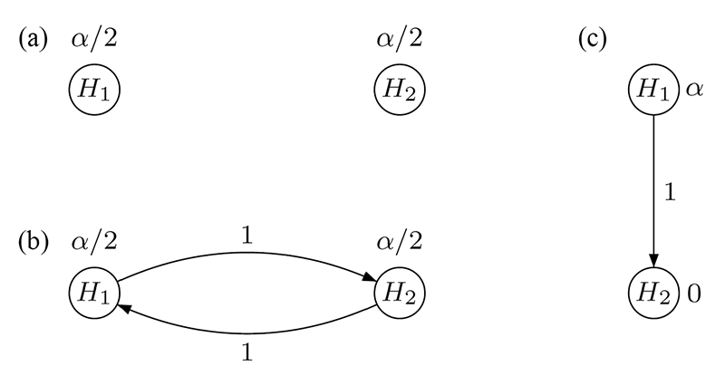
Figure 1. Graphical visualization of (a) the Bonferroni method, (b) the Holm procedure, and (c) the hierarchical test procedure, each for two null hypotheses H1 and H2.
As for any graphical test procedure, the hierarchical test procedure controls the FWER and is often used in practice because it allows reflecting study objectives of unequal importance.
The advantages of graphical test procedures become evident when multiple sources of multiplicity have to be addressed within a single study. Using the ideas above, it is possible to flexibly combine “horizontal” Bonferroni-based test strategies as in Figure 1(a) and 1(b) with “vertical” hierarchical test strategies, as in Figure 1(c), into a single graphical multiple test procedure that is tailored to the given structured study objectives.
To illustrate this flexibility, consider the problem of comparing both low and high dose of the new drug against the placebo for FEV1 and time-to-exacerbation. Suppose that the latter outcome variable is assessed based on pooling the data across both doses because each individual dose-placebo comparison is assumed to be underpowered on its own. Thus, there are three null hypotheses H1, H2 (comparing low and high dose against placebo for FEV1, respectively), and H3 (comparing the pooled doses against placebo for time-to-exacerbation).
Reflecting clinical considerations, the three hypotheses are not considered equally important (where, again, the importance relationship is a result of ordering the trial objectives subject to various considerations, as explained above): The secondary hypothesis H3 is tested only if at least one of the two primary hypotheses H1 and H2 have been rejected first.
Common multiple test procedures could be applied, but these may not reflect the relative importance of the three hypotheses. For example, the Bonferroni test would treat FEV1 and time-to-exacerbation as equally important and thus not reflecting the relative hierarchy. Likewise, the hierarchical test procedure would reflect the relative importance of both variables, but not be able to incorporate the two dose-placebo comparisons for FEV1.
Consider, in contrast, the graphical test procedure visualized in Figure 2(a). Initially, H1 and H2 are each tested at local level α/2, while H3 is assigned level 0. Suppose that H1 can be rejected (i.e., p1 ≤ α/2). Then, its level α/2 is split evenly and propagated so the remaining hypotheses H2 and H3 can be tested at the updated levels of 3α/4 and α/4, respectively; see Figure 2(b). The converse is also true if H2 is rejected first. After updating the graph according to a specific algorithm, testing continues with the remaining primary hypothesis and H3: If either of these two hypotheses is rejected at its local significance level, the last remaining hypothesis is tested at full level α.
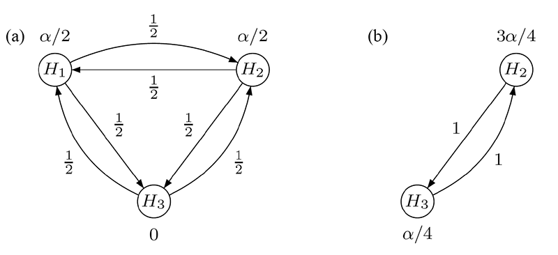
Figure 2. Graphical multiple test procedure for two primary and one secondary hypothesis: (a) initial graph,
(b) updated graph after rejecting H1.
The last example illustrates that graphical approaches offer the possibility to tailor advanced multiple test procedures to structured families of hypotheses and visualize complex decision strategies in an efficient and easily communicable way while controlling the FWER at a designated significance level α.
When Convention Meets Practicality
The considerations in the previous section focus on multiplicity challenges arising within a single clinical study, such as comparing several doses of a new drug for more than one outcome variable. A different source of multiplicity arises when evidence is collected from multiple studies.
For example, it is common practice to request two statistically significant confirmatory Phase III clinical studies (the so-called two-study convention), which provides a stringent replicability standard in pharmaceutical drug development. Phase III studies are usually designed with large sample sizes to provide sufficient exposure of the new drug in the target population. As a result, managing two large, long-term studies may pose logistical and practical challenges.
The following case study illustrates the specific challenges when thinking “outside the box” and convention meets practicality.
The initial consultancy request involved how to design the Phase III studies to confirm the efficacy of a new drug under development, compared with a placebo. The new drug was intended to treat a disease with an unmet medical need. Given the conventional framework, two identical studies were planned with the same sample size to measure the same outcome variables.
More specifically, three clinical outcomes were considered: (1) reduction of a short-term symptom, (2) reduction of a long-term symptom, and (3) a variable measuring improvement of patients’ quality of life.
Because the short-term symptom (1) is used conventionally for regulatory purposes to decide whether the new drug is effective, it was designated by the clinical team as the primary variable. On the other hand, it was acknowledged that the long-term symptom (2) and the quality of life variable (3) were more closely related to improving patients’ daily life and thus designated as secondary variables that had to be included in the multiple testing considerations. As suggested by regulatory guidelines governing clinical drug development, the FWER had to be controlled at level α for the entire family of hypotheses corresponding to the primary variable (1) and both secondary variables (2) and (3).
Based on the relative importance of each variable, the clinical team initially considered applying separate hierarchical test procedures for the two confirmatory studies. Figure 3 visualizes the two test hierarchies, one for each study, with the test sequences H1 → H2 → H3 and H'1 → H'2 → H'3. Note that for each i = 1,2,3 the hypotheses Hi and H’i are, in fact, the same, using the prime notation only to distinguish between the studies.
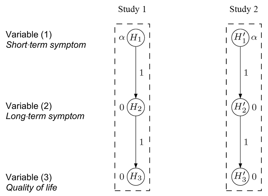
Figure 3. Separate hierarchical test procedures for two confirmatory studies.
After completing the studies and conducting the individual study-level analyses, success for a variable can be claimed only if it is significant in both studies, reflecting the replicability criterion that follows from the two-study convention mentioned above. For example, benefit on variable (1) is claimed only if both H1 and H'1 are statistically significant, each at level α.
While the story could end here as a simple illustration of the graphical approach, the challenge just begins. Based on the sample size calculation for each study, the clinical team would need about 1,000 patients to achieve an adequate power on variables (1) and (3), but 2,000 patients for variable (2). This means 2,000 patients would have to be recruited in total for each study, which takes about five years to complete.
In practice, it would be challenging, perhaps even impossible, to run two long-term studies of this size in this indication. Thus, the follow-up question was whether the data could be used more efficiently to shorten the duration of the study, while still maintaining the replicability standard.
One immediate approach is to pool the data from the two identical studies and adjust for potential differences using “study” as a stratification factor. For the case study at hand, the data are pooled for variable (2) but still assess variables (1) and (3) separately for each study, resulting in the test procedure conceptualized in Figure 4. If the hypotheses H1 and H'1 are both significant, each at level α, there is enough evidence to support efficacy on variable (1) based on the results from the two replicated studies.
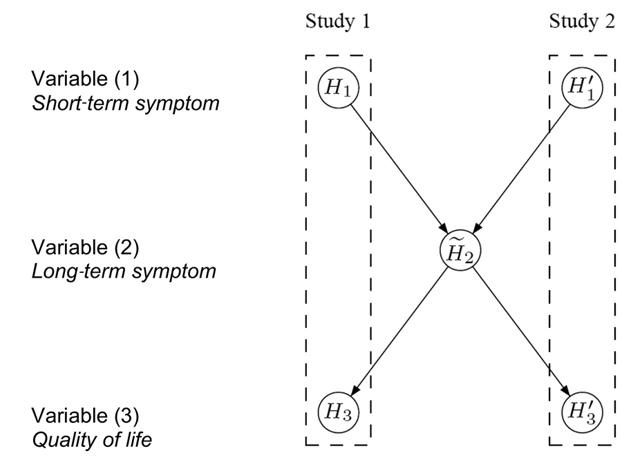
Figure 4. Conceptual visualization of a hierarchical test strategy, using the pooled data for H̃2. Details about its interpretation are in the text.
The hypothesis H̃2 is then tested at level α using the pooled data from both studies. If H̃2 is also rejected, H3 and H'3 are tested separately at level α. Success can only be claimed on variable (3) if both H3 and H'3 are significant. Note that Figure 4 visualizes the hierarchical test strategy on a conceptual level, in contrast to the graphs in Figures 1–3, which can be used as formal inferential tools.
It is easy to communicate the test procedure conceptualized in Figure 4 with clinical teams and regulatory agencies. The sample size is reduced by half and similarly, the duration of the studies is shortened considerably. However, this strategy still bears a major practical challenge: Analyzing the null hypothesis H̃2 using the pooled data would require both studies to be completed at the same time.
If, by chance, one study is delayed, the result on H̃2 is also delayed. Consequently, the analysis of the other study cannot be completed either because the testing for H3 and H'3 depends on the result for H̃2 and, ultimately, on the delayed study.
To allow efficient execution of the two studies, the test procedure conceptualized in Figure 5 was recommended in the end to the clinical team. In each study, the hypotheses (H1 and H3, or H'1 and H'3) are tested separately in a hierarchical order at level α. That is, if we can reject H1 (or H'1) at level α, then we can continue testing H3 (or H'3) at level α. If both H1 and H'1 are statistically significant, replicability is established and the pooled analysis for H̃2 can be carried out.
Similarly, a claim of success with respect to both H3 and H'3 is only made if they are rejected in both studies. The significance level for testing H̃2 is α – α2, as a result of a Bonferroni split between H3, H'3 and H̃2, after significant results for H1 and H'1. Since the two tests for H3 and H'3 are stochastically independent, the Type I error rate to reject both at level α is at most α2.
On the other hand, if only the pooled analysis were done, its significance level would be α. Thus, the remaining significance level assigned to H̃2 is α – α2.
This test procedure guarantees the control of various Type I error rates as follows:
- The FWER rate for each study; i.e., for each of the two hypothesis families {H1,H3} and {H’1,H'3}, is controlled at level α.
- The Type I error rate for the primary variable (1) is controlled at level α2 because H1 and H'1 each has to be rejected at level α, using independent tests, to claim an effect on the short-term symptom.
- The FWER for the secondary variables (2) and (3) is controlled at level α. In particular, H̃2 has to be rejected at level α – α2 to claim an effect on the long-term symptom, conditional on having rejected H1 and H'1 before. Similarly, H3 and H'3 each has to be rejected at level α to claim an effect on the quality of life variable, again conditional on having rejected H1 and H'1.
After communicating with the clinical study team and regulatory agencies worldwide, the graphical test procedure from Figure 5 was accepted and implemented. Note that Figure 5 again visualizes the test strategy on a conceptual level, in contrast to the formal graphs used in Figures 1–3.
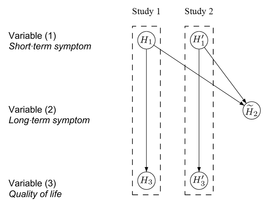
Figure 5. Conceptual visualization of a hierarchical test strategy with separate testing of H̃2 using the pooled data. Details about its interpretation are in the text.
Discussion
Drug development encompasses a series of several dozens of preclinical and clinical studies, each generating new data and creating the need for making decisions in the face of uncertainty. As a consequence, drug development is prone to a lack of replicability if not addressed carefully.
Multiplicity, in particular, raises challenging problems that affect almost every decision throughout drug development. Different stages of drug development are subject to different requirements (including regulatory and industry perspectives) and might need different solutions. Good decision-making has to account for multiplicity, where it is critical to choose the most suitable method for a particular problem.
There is no single “black-box” tool to address multiplicity. Strong statistical leadership is required to guide multidisciplinary teams to elicit the underlying study objectives and their relative importance to each other, along with understanding the practical and logistical constraints, creating the need to search for tailored multiple test strategies that enable the design and planning of scientific research to facilitate accurate interpretation of results and good decision-making based on data.
Further Reading
Bretz, F., Maurer, W., Brannath, W., and Posch, M. 2009. A graphical approach to sequentially rejective multiple test procedures. Statistics in Medicine 28(4), 586–604.
Bretz, F., and Westfall, P.H. 2014. Multiplicity and replicability: Two sides of the same coin. Pharmaceutical Statistics 13, 343–344.
Ioannidis, J.P.A. 2005. Why Most Published Research Findings Are False. PLoS Medicine 2(8): e124.
Tukey, J.W. 1977. Some thoughts on clinical studies, especially problems of multiplicity. Science 198: 679–684.
About the Authors
Frank Bretz is a Distinguished Quantitative Research Scientist at Novartis. He has supported methodological development in various areas of pharmaceutical statistics, including dose finding, multiple comparisons, estimands, and adaptive designs. He currently holds adjunct/guest professorial positions at the Hannover Medical School (Germany) and the Shanghai University of Finance and Economics (P.R. China).
Willi Maurer was the head of biostatistics at Novartis and founded its Statistical Methodology group, which he led until his retirement in 2006. He then served as a senior statistical consultant to the group. He was interested in the development and implementation of novel statistical methodologies related to multiplicity and adaptive designs, especially under the interdisciplinary, ethical, economical, and regulatory challenges that drug development is faced with during the design, analysis, and interpretation of clinical trials. He died while this manuscript was under revision. We are indebted to him as our colleague, mentor, and friend.
Dong Xi is associate director of the Statistical Methodology group at Novartis. He has supported the development and implementation of innovative statistical methodology in multiple comparisons, dose finding, and group sequential designs, and has provided consulting and simulation support in various therapeutic areas.


