
Epic Fail? The Polls and the 2016 Presidential Election

Donald Trump’s victory in the 2016 presidential election caused widespread shock, in large part because political polls seemed to predict an easy victory for Hillary Clinton. New York magazine was so confident of a Clinton victory that, the week of the election, its cover featured the word “loser” stamped across Donald Trump’s face.
The day after the election, Politico asked, “How Did Everyone Get It So Wrong?” The next month, a columnist for the New Republic asked, “[A]fter 2016, can we ever trust the polls again?” given that they “failed catastrophically” in the presidential race. A Wall Street Journal columnist doubtless referred to the 2016 outcome when he noted that recent election polls had been “spectacularly wrong.”
Was the primary failure among the polls or, instead, among Americans who, for whatever reason, were unable to recognize what the polls were actually saying? We explore the issue by considering two primary consolidators of presidential polls: FiveThirtyEight.com, the Nate Silver website that was previously considered the gold standard among consolidators, and Real Clear Politics, the immensely popular political website that had 32 million unique visitors in the month before the 2016 election.
It is of interest to know what these consolidators reported on the eve of the election, and then consider what their forecasts implied about polling accuracy in key states that were credited or blamed for Hillary Clinton’s “reversal of fortune.”
Properly understood, the publicly available polls suggested that the Clinton/Trump race was what the media, in comparable circumstances, would typically call a “statistical dead heat.” The belief that the Democrat was all but certain to win was inconsistent with both a superficial awareness of what the polls said and a deeper understanding of what they implied about the outcome.
To the question “Can we ever trust the polls again?” after what happened in 2016, the answer is an emphatic yes.
On Election Day
Even a cursory look at FiveThirtyEight or Real Clear Politics on the morning of Election Day 2016 would have suggested that a Clinton victory was far from inevitable. In its poll-based forecast, FiveThirtyEight estimated then that Trump had a 28.6% chance of winning the presidency. Real Clear Politics predicted that the Electoral College breakdown of the results would be 272 for Clinton and 266 for Trump.
That prognosis implied that, if only one state switched from Clinton to Trump, Trump would be president. Even if the switching state had only three electoral votes (the minimum number), the result would be a 269–269 tie, in which case, Trump would prevail when the winner was chosen by the Republican House of Representatives.
To be sure, on Election Day itself, many people were no longer looking at polls, but polling outcomes a few days before the election were, if anything, more favorable to Trump: On November 4, 2016, for example, FiveThirtyEight estimated Trump’s chances of winning four days hence at 35.4%. Thus, evidence of a close race cannot be said to have arisen too late to be widely noticed.
Paradoxically, respect for the two consolidators and the state-specific polls they summarized actually grows if one looks further at what they supposedly did wrong.
FiveThirtyEight’s “Errors” in Three Key States
The great surprise in the 2016 election was that Donald Trump carried Pennsylvania, Michigan, and Wisconsin, three states that were considered part of the Democratic “firewall.” FiveThirtyEight did not contradict the general impression: Its polls-only forecast the morning of the election was that Trump had a 21.1% chance of winning Michigan, a 23.0 chance of winning Pennsylvania, and a 16.5% chance of carrying Wisconsin. (Those “polls-plus” forecasts that also considered economic and historical factors were essentially the same.)
A simple calculation with the FiveThirtyEight estimates might suggest that Trump’s chances of achieving a “trifecta” in these states was essentially .211 ∗ .23 ∗ .165 = 1 in 125, but such a calculation would be unfair to FiveThirtyEight.
Advancing the statistic “1 in 125” is misleading for two reasons. The first is that judging a forecasting model by what emerged as its weakest forecasts is systematically biased against it. The second is that the calculation treats the three outcomes as independent, when FiveThirtyEight explicitly assumes that they are not. Although its specific procedures are not transparent, FiveThirtyEight recognized that the outcomes in these three similar states are correlated. Indeed, on election night, TV commentators readily grasped that Trump’s strong performance in Pennsylvania increased the chance that he would also carry Michigan and Wisconsin.
A simple analysis indicates the strength of the pattern of correlation. Assuming that FiveThirtyEight’s probability assessments were accurate in Pennsylvania and Wisconsin (at 23.0% and 16.5% for Trump, respectively), how might one estimate the chance that he would win in both states?
One reflection of the correlation is that, in the 12 elections before 2016, Pennsylvania and Wisconsin went for the same candidate 10 times (whether Republican or Democrat, and whether the national winner or the national loser). Using this statistic, we can set up some simple equations that approximate the chance that Trump would carry the two states.
Some definitions:
PCC = probability that Clinton would win both Pennsylvania and Wisconsin
PTT = probability that Trump would win both Pennsylvania and Wisconsin
PCT = probability that Clinton would win Pennsylvania and Trump would win Wisconsin
PTC = probability that Trump would win Pennsylvania and Clinton would win Wisconsin
On the morning of the election, we could write:
PCC + PTT = 10/12 (based on the historical chance both states go the same way)
PTT + PTC = .230 (based on FiveThirtyEight’s forecast of the chance Trump would win Pennsylvania)
PTT + PCT = .165 (based on FiveThirtyEight’s forecast of the chance Trump would win Wisconsin)
PCC + PTT + PCT + PTC = 1 (because something has to happen)
Solving this system of linear equations provides:
PTT = .114 PTC = .116 PCT = .051 PCC = .719
That PTT = .114 (as opposed to .23 ∗ .165 = .038) implies that the tendency of Pennsylvania and Michigan to “go the same way” yields a much greater chance of a double victory than would arise under the FiveThirtyEight projections and an independence assumption. The chance that Trump would carry at least one of the states would be estimated by 1 – .719 = .2.
What about Michigan, as well as Pennsylvania and Wisconsin? The historical pattern is that, over the 12 presidential elections from 1960 to 2012, Michigan went along with Pennsylvania and Wisconsin every time the latter two states voted for the same candidate (i.e., 10 times out of 10). It therefore could be approximated:
PTTT = P(Trump would win PA, MI, and WI) ≈ P(win PA and MI) ∗ (10/10) = .114
and:
P(Trump win at least one of PA, MI, and WI) ≈ 1 – P(Clinton wins all three).
or P(Trump win at least one of PA, MI, and WI) ≈ 1 – .719 ∗ (10/10) = .281
These calculations, however, do not actually use FiveThirtyEight’s estimate that Trump’s chance of carrying Michigan was .211. One could perform the analogous calculations based initially on Pennsylvania plus Michigan, and on Michigan plus Wisconsin, as shown in Table 1.
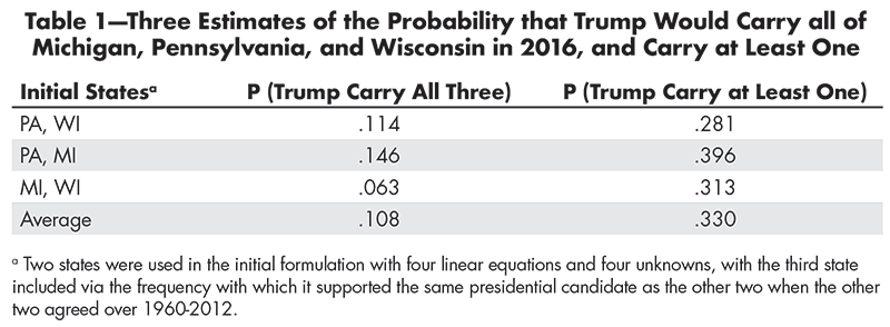
Table 1—Three Estimates of the Probability that Trump Would Carry all of Michigan, Pennsylvania, and Wisconsin in 2016, and Carry at Least One
The key probabilities exhibit some variation over the three approximations, but the collective results suggest roughly a 1 in 9 chance that Trump would win all three states, and about a 1 in 3 chance that he would carry at least one. (The use of an omnibus linear model that considers all three of FiveThirtyEight’s projections at once—with eight equations and eight unknowns—does not yield more reliable probability estimates than the three-part approximation above.)
This 1 in 3 probability is especially noteworthy because, outside PA, MI, and WI, Trump amassed 260 electoral votes. That outcome was very much consistent with the state-by-state projections by both FiveThirtyEight and Real Clear Politics, but, once Trump had 260 electoral votes, he only had to win one of PA/MI/WI to achieve a national victory. If the chance of that outcome was something like 33%, it is no surprise that FiveThirtyEight saw a probability near 3 in 10 that Trump would triumph.
The Democratic “firewall” was far from fireproof.
These probability calculations are obviously approximate, and weigh historical patterns almost as much as the individual FiveThirtyEight projections, but the general point of the exercise survives its imperfections. There was reason to believe that, if Trump performed better than expected in one of the three states, he was more likely to do so in the others. Because FiveThirtyEight gave Trump an appreciable chance of winning each of the three states and recognized that the outcomes were not independent, it saw a Clinton victory as far from a sure thing—and it did so based largely on in-state polling results, which by no means deserved to be described as “spectacularly wrong.”
Real Clear Politics
As noted, Real Clear Politics (RCP) predicted on Election Day that Trump would get 266 electoral votes, compared to Clinton’s 272. It correctly identified the winner in 47 of the 51 states, erring—like FiveThirtyEight—in PA, MI, and WI, and also in Nevada. (FiveThirtyEight got Nevada right, but it tilted toward Clinton in Florida and North Carolina, which she lost.) However, RCP listed all four of the states it got wrong in its “tossup” category.
Still, the specific procedure by which RCP assigned a state’s winner would cause statisticians to tear their hair out. Roughly speaking, it considered all major polls in the state within two weeks of the election, and took a simple arithmetical average of their results. If Trump was ahead of Clinton in this average, he was awarded the state in RCP’s “no tossup” assessment.
The procedure obliterated the distinction between:
- A poll one day before the election and another 13 days before
- A poll with sample size 1,500 and another with sample size 400
- A poll among all registered voters and another restricted to “likely” voters
Furthermore, RCP assigned no margin of error to its state-specific forecasts.
It is desirable to place the RCP results on a stronger statistical foundation, especially as an indicator of the caliber of state-level polls that it summarized. A simple way to do so is to accept RCP’s assumption that the various polls in its average are essentially interchangeable. A “megapoll” could be created by combining all the individual polls RCP used for a given state in its Election Day forecast. Using that megapoll, one can estimate a margin of sampling error for the statewide result and—more importantly—estimate the probability that Trump would carry the state.
For example, the final 2016 RCP poll listings for the state of Ohio are shown in Table 2.
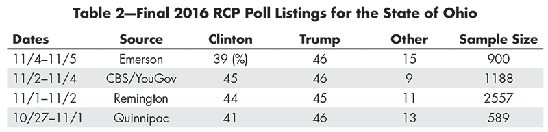
Table 2—Final 2016 RCP Poll Listings for the State of Ohio
(It was not RCP that rounded-off polling results to the nearest percentage point; rather, that convention was followed by all four polls in their announcements of the results.)
Trump’s average lead over Clinton in the four Ohio polls (weighed equally) was 14/4 = 3.5 percentage points, and that was the statistic featured by RCP in its summary about Ohio.
Although an average of 12% of those canvassed in the four polls were either undecided or supportive of a third-party candidate, the tacit assumption was that such voters could effectively be ignored in the race between Clinton and Trump.
The Emerson poll in Ohio generated 900 ∗ .39 = 351 supporters of Clinton and 900 ∗ .46 = 414 of Trump. For CBS/YouGov, the corresponding numbers were 546 and 535. For the four merged polls, Clinton had 2,252 supporters while Trump had 2,382. Obviously, the large Remington poll had a disproportionate effect on the merged result. If no relevance is accorded to the identity of the pollster, though, the number of days until the election, and the likelihood a polled voter will actually vote, then one can presumably construe the Clinton/Trump result in Ohio as arising from a random sample of 2,252 + 2,382 = 4,634 voters.
Among such voters, Trump’s share of the Clinton/Trump vote was 51.4% and Clinton’s was 48.6%.
Taking sampling error into account, what is the probability that Trump was actually ahead in Ohio, given the result of the “megapoll?” Starting with a uniform before Trump’s vote share versus Clinton and revising it in Bayesian manner with the findings for the 4,634 voters sampled, the chance that Trump would defeat Clinton in Ohio would be estimated as .972. (This result arises from a beta distribution with α = 2,383 and β = 2,253.)
Proceeding similarly, one can get a poll-based estimate of the chance that Trump would win in each of the 51 states.
An RCP Projection
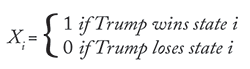
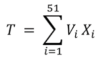
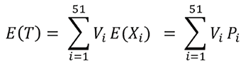
If Vi is state i’s number of electoral votes (i = 1, .., 51) and the indicator variable Xi is defined by:
then T—Trump’s total number of electoral votes—follows:
Then, if Pi = P(Trump will win state i | recent polling results there), the mean of T is given by:
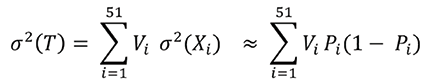
RCP never mentions possible correlations among the Xi‘s, and tacitly treats the Xi‘s as independent (implying that similarities across states are already appropriately reflected in the point estimates of the Xi‘s). Under independence, the variance of T would approximately follow:
To estimate P(Trump wins) = P(T ≥ 269 out of FiveThirtyEight Electoral Votes), we might be tempted to assume that T is normally distributed as the sum of 51 independent random variables. However, the heavy majority of Pi‘s (calculated with the method shown above for Ohio) are very close to either zero or one. As a practical matter, therefore, the uncertainty in T depends on a small subset of the state-specific variables.
Thus, to approximate P(Trump wins), we turn to simulation rather than treat T as normal, using the calculated Pi‘s = 258.8, with a standard deviation of about 17.3.
More than 2,000 simulation runs using the state-specific Pi‘s, the fraction in which Trump was victorious was .290. This estimate of P(Trump wins) might seem smaller than expected given RCP’s estimated 266–272 split. But, as the value of E(T) suggests, Trump was only modestly ahead in several states assigned to him (i.e., several of his Pi‘s only moderately exceeded 1/2), while Clinton’s leads were more substantial in the states where she led.
What should we make of the estimate that P(Trump wins) ≈.290 (which, coincidentally, is very similar to the estimate made by FiveThirtyEight)? Consider a pre-election poll that suggests that candidate A leads candidate B by 51% to 49%, with a margin of error of 3 percentage points. The media would routinely describe the race as “a statistical dead heat” or at least “too close to call.” If, on Election Day, candidate B were to win with 50.3% of the vote, few people would cite the result as evidence that the poll was wrong.
This point is relevant because, under the standard formula for a 95% confidence interval, the sample size in this hypothetical poll with its 3-percentage-point error margin would be 1,068, and the split corresponding to 51%/49% would be 544 for A and 524 for B. Under a Bayesian revision of a uniform prior, B’s true share of the vote would follow a beta distribution with α = 525 and β = 545 ), and the chance that B was actually ahead would be estimated as 25.0%.
An obvious question arises: If a poll is not seen as inaccurate when it had assigned the actual winner a 25.0% chance of victory, how can one say that RCP was “spectacularly wrong” when it implied a 29.0% probability that Trump would win the presidency?
Indeed, in a two-candidate race with no undecided voters and a poll with a 3-percentage-point margin of error, the outcome would be treated as “too close to call” if B’s estimated vote share was anything above 47%. But that means that the race would be viewed as undecided even when B’s approximate chance of actually winning was as low as .03. The observed split corresponding to a 29% chance that B would win would be 50.8% for A and 49.2% for B, and the split—which obviously suggests a close race—is statistically equivalent to the result implied by Real Clear Politics in 2016.
The good performance of RCP—despite ignoring the correlation among outcomes in PA, MI, and WI—is quiet testimony to the high accuracy of the individual polls it synthesized.
If the conventional wisdom is that the polls failed in 2016 systematically, then the conventional wisdom is somewhat more in error than the polls were.
In Conclusion
The day after the election, the New York Times ran the headline “Donald Trump’s Victory Is Met with Shock Across a Wide Political Divide.” That assessment was clearly accurate but, as we have suggested, this “shock” should be viewed as arising less because of the polls than despite them. Ironically, the real lesson from 2016 could be that not that we should pay less attention to the polls, but that we should pay more attention.
Further Reading
Caldwell, C. 2017. France’s Choice: Le Divorce? Wall Street Journal.
FiveThirtyEight. 2016. Who will win the presidency?.
Healy, P., and Peters, J. 2016. Donald Trump’s Victory Is Met with Shock Across a Wide Political Divide. New York Times.
Narea, N. 2016. After 2016, Can We Ever Trust the Polls Again? New Republic.
Real Clear Politics, 2016 Presidential Election, No Toss-Up States.
Vogel, K., and Isenstad, A. 2016. How Did Everyone Get It So Wrong? Politico.
About the Author
Arnold Barnett is the George Eastman Professor of Management Science and professor of statistics at MIT’s Sloan School of Management. He has received the President’s Award for “outstanding contributions to the betterment of society” from the Institute for Operations Research and the Management Sciences (INFORMS), and the Blackett Lectureship from the Operational Research Society of the UK. He has also received the Expository Writing Award from INFORMS and is a fellow of that organization. He has been honored 15 times for outstanding teaching at MIT.
It was interesting to read at the bottom of the polls I looked at that Democrats were consistently over-polled by from 5% to 15%. Two things went through my mind at the time: Where’d they get those baloney numbers from that there were 15% more registered Democrats than Republicans, and why would they tell us that they were cooking the books by using inflated populations?
My guess to the first is that they were so in bed with Hillary – perish the thought, not even Bill is in bed with Hillary – that they couldn’t ‘bare’ the thought that the queen has no clothes, so they fudged the data enough to make it look like she was dressed in purple and awaiting her due at coronation.
To the second, I have NO idea.