
Zika Is Here, and We Need Statistics
A new virus du jour is sending epidemiologists and statisticians across the world into a frenzy. Its name is Zika. Headlines continually blare things like “State health officials urged to get ready for Zika in the United States” and “Zika could make America’s contraception failures even worse.” Scientists continue to grapple with the potential magnitude of the Zika outbreak, which is considerably challenging to gauge based on existing data, due to a number of uncertainties that cloud the relationship between observed cases and true infections.
The Zika virus is a mosquito-borne pathogen that is rapidly spreading across the Americas. Although the Zika virus symptoms are mild, the virus can have drastic implications for newborns. Due to a probable association between Zika virus infection and a congenital neurological disorder called microcephaly (see box), the epidemic trajectory of this viral infection poses a significant concern for the nearly 15 million children born in the Americas each year. The need for a more accurate and predictive approach in mathematical modeling of diseases like Zika is pressing.
A Little History
When Ronald Ross tipped over the water tank outside his cottage in Bangalore, it began his lifelong battle against mosquitoes. It was 1883 and Ross, only two years out of medical school, was the British Army’s new garrison surgeon. Overall, he was happy with the posting—he considered the city, with its sun, gardens, and villas, to be the best place to live in southern India.
He was less enthusiastic about the mosquitoes. Having arrived to find his room filled with the sound of their buzzing, he decided to hunt down and destroy their breeding grounds in pools of stagnant tank water. The plan worked: As he drained the tanks, mosquito numbers fell.
The longer Ross spent in the region, the more he began to suspect that those mosquitoes transmitted malaria, an often-lethal disease with spiking fevers and other symptoms resembling a devastating flu. Its name came from Renaissance Italy; mala aria, or “bad air,” referred to the suspected cause of the disease.
To prove the connection between mosquitoes and malaria, Ross experimented with birds. He allowed mosquitoes to feed on the blood of an infected bird and then bite healthy ones. Not long afterward, the healthy birds came down with the disease, too. To verify his theory even further, Ross dissected the infected mosquitoes, and found malaria parasites in their saliva glands. Those parasites turned out to be Plasmodium, identified by a French military doctor who had discovered the virus in the blood cells of infected patients a few years earlier.
Next, Ross wanted to show how the disease could be stopped, and his experiment with the water tank paved the way. Get rid of enough insects, he reasoned, and malaria would cease to spread. To prove his theory, Ross, a keen amateur mathematician, constructed a theoretical model—a “mosquito theorem”—outlining how mosquitoes might spread malaria in a human population. He split people into two groups—healthy or infected—and wrote down a set of equations to describe how mosquito numbers would affect the level of infection in each.
The human and mosquito populations formed a cycle of interactions: The rate at which people became infected depended on the number of times they were bitten by infected mosquitoes, which depended on how many such mosquitoes there were, which depended on how many humans had the parasite to pass back to those mosquitoes, and so on. Ross found that, for the disease to persist steadily in a population, as it did in India, the number of new infections per month would have to be equal to the number of people recovering from the disease.
Using his model, Ross showed that it was not necessary to remove every mosquito to bring the disease under control. Destroy enough mosquitoes, and people infected with the parasite would recover before they were bitten enough times for the infection to continue at the same level. Therefore, over time, the disease would fall into decline. In other words, the infection had a threshold, with outbreaks on one side and elimination on the other.
Ross’s work, which won him a Nobel Prize in 1902 and a knighthood in 1911, set the stage for a new mathematical way of thinking about disease outbreaks from bubonic plague to influenza. His insight influenced vaccine policy through the concept of “herd immunity”: Vaccinate a sufficient proportion of the population, and the disease will not turn into an epidemic.
This means that vaccination can work even if a few people are left unprotected. Although the specific control measure is different—giving vaccines rather than removing mosquitoes—the principle is the same. As long as we remove enough links in the chain of events that generate infections, the disease will die out. It is not necessary to vaccinate everyone, or remove every mosquito; if we reach the critical threshold, the infection will struggle to cause outbreaks in the population.
Bottom of Form
Other researchers studied infections in a mathematical way before Ronald Ross, but their approaches focused on past events. Take the physician John Snow, who used logical reasoning to trace the cause of the 1854 London cholera outbreak. As with malaria, most people at the time blamed cholera on “bad air,” but when Snow plotted the locations of all disease cases on a map, he noticed that the water pump on Broad Street in London was the local water source for infected households. He reasoned that patients were catching cholera from contaminated water, which meant that removing the source on Broad Street would halt the spread of the disease.
Rather than look backward, Ross looked ahead, and his enthusiasm for predicting the future convinced colleagues to join in. One was a young mathematician named Anderson McKendrick, a member of the Indian Medical Service Ross had met during an anti-malarial campaign in Sierra Leone. McKendrick came down with a tropical gut disease in 1920 and, like Ross before him, ultimately left India. When he returned to Edinburgh, he took a position at the Laboratory of the Royal College of Physicians. There he met William Kermack, a chemist who was also interested in infectious diseases.
Together, they extended Ross’s method of examining the interactions that drive epidemics. Along with looking at infections that simmered away over time, such as malaria, McKendrick and Kermack studied diseases such as the plague, which exploded through a population before disappearing again.
Like Ross, they grouped the hypothetical population into groups that were healthy or infected. But this time there were no mosquitoes: The infection spread directly from person to person. As before, individuals started out susceptible to infection. Upon exposure, they would move into the infectious group. Finally, they would leave the infectious group, either because they had gained immunity to the disease (a reasonable assumption for infections such as measles and pandemic flu) or because they had died (as was common with the plague).
In general, this mathematical framework is denoted as a compartment model in epidemiology, where “group” is synonymous with “compartment”—and members are typically assigned letters (“S” susceptible, “I” infectious, etc.—the SIR model). The way that these compartments interact is often based on subjective assumptions, and the model is built up from there.
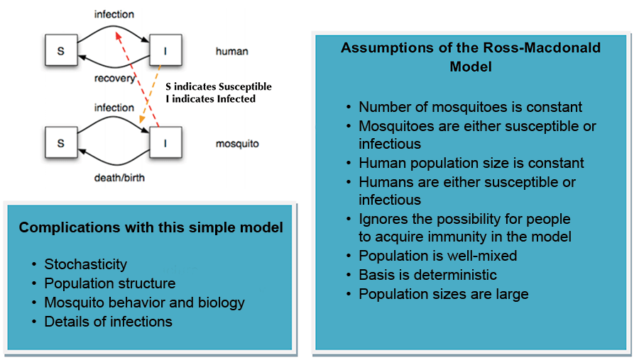
Figure 1. The Ross-Macdonald Model with assumptions and complications.
These models are usually investigated through ordinary differential equations (which are deterministic), but can also be viewed in a more realistic stochastic framework. To push these basic models to further realism, other compartments are often included, most notably the recovered/removed/immune compartment.
Although the most common compartment model is the SIR model, the models can gain many more letters—symbolizing even more compartments/possible states for people. A popular model for Ebola was Legrand’s ¥ Susceptible – Exposed – Infected (at Home) – Infected (at Hospital) – Infected (at Funeral) – Removed (SEIHFR) model, due to the multiple infectious states that Ebola has (I when at home, H in hospital, and F at a funeral). These additional compartments simulate Ebola-specific paths of transmissions; the disease was often spread while people were being treated in hospitals or after they touched bodies at a funeral. Models can get very complicated, as seen in that by Pandey (Figure 2).
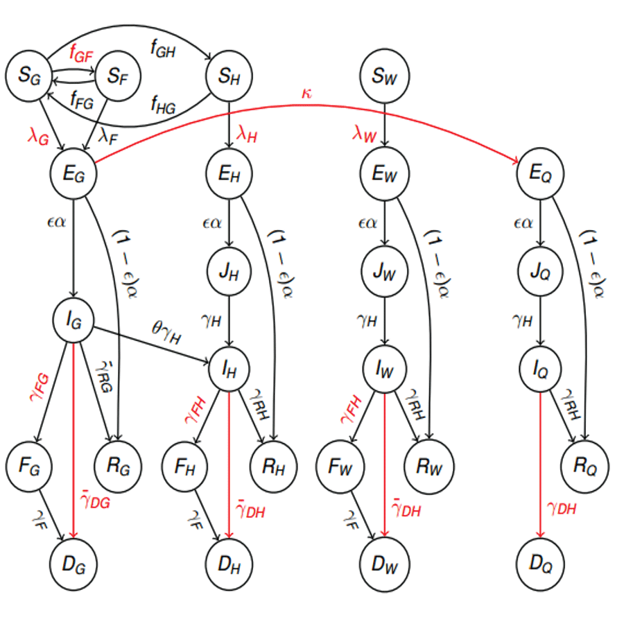
Figure 2. An extremely complex model by Pandey, et al., and Harling—our continuous-time stochastic model of Ebola transmissions between and within a community, hospitals, and funerals. It tracks the number of people who are susceptible (S); latently infected (E); infectious (J & I); deceased Ebola victims buried in traditional West African funeral customs (F); buried Ebola victims (D); and recovered with immunity (R). We also distinguished between individuals who have different levels of exposure to Ebola, based on whether they are part of the general community (subscript G), hospitalized for a reason other than Ebola (H), healthcare workers (W), attending a funeral ceremony (F), or quarantined (Q).
This diagram shows the per-capita transition rates between compartments, with red labels indicating rates that can be affected by interventions and red arrows indicating rates that are entirely due to interventions. The J compartments ensure that the duration of infection for hospitalized Ebola victims is the same whether they were infected in the community or the hospital. The forces of infection are functions of the number of infectious people, as are the transition rates ƒGF to funerals, ƒGH to hospitalization, and to quarantine.
These models sacrifice simplicity but allow you to track everything with great care. To summarize, we have boxes (in the case above—circles) and then arrows that show transitions between each box.
It should be emphasized that one cannot think of compartments and the flows in and out of compartments as individual components in which each part can be described independently of each other. Both the inflow and the outflow from any compartment may depend on the volume inside the compartment. Similarly, the inflow into a compartment may be dependent on the outflow from another compartment.
In other words, it is important to think of the system as a whole, in which the parameter representing the material in the compartment (the state-variable) can depend on what flows in and what flows out.
In addition, since what flows into one compartment typically flows out of another compartment, the variables depend on each other and on the state of the system as a whole. The important point to remember is that it is the person modeling the system who chooses how the model parameters and variables depend on each other.
Progress was not always smooth. In 1924, Kermack was blinded in a lab accident, so from that point onward, he performed all of his calculations in his head. He and McKendrick eventually published their findings in 1927 in a paper entitled “A Contribution to the Mathematical Theory of Epidemics” in the Proceedings of the Royal Society of London. This paper tackled one of the most important questions in epidemiology: What causes an epidemic to end?
From influenza to the plague, the number of cases in a real epidemic often rises exponentially at first. After awhile, the disease reaches a peak level, and then the number of new cases starts to decrease. When McKendrick and Kermack began their research, people generally gave two possible reasons for the decline: The epidemic faded away either because the infection had become less potent over time, or because there were no susceptible people left—everyone had been infected and either died or became immune.
In their model, McKendrick and Kermack assumed that the pathogen stayed the same throughout the epidemic; the infection did not weaken over time. Yet, the model still produced an eventual decline in cases. When the pair compared the model to the 1905 outbreak of the plague in Bombay, the predicted number of cases closely matched the real disease level.
Was the decrease in infection caused by a lack of susceptible people? Apparently not: In the model, some susceptible individuals always remained at the end of the outbreak. McKendrick and Kermack demonstrated that epidemics do not necessarily decline because everyone has been infected. They can also end because there are not enough infected people left to sustain transmission. Once enough people are immune, infected individuals are unlikely to meet other susceptible people, which means that they generally recover before infecting others.
This effect is inevitable in the later stages of an outbreak, but it is also possible to force an epidemic into this situation. In Ross’s model, the reduction in infection came from getting rid of mosquitoes. During a vaccination campaign, it comes from targeting a large portion of the susceptible population.
It would be decades before the next major breakthrough in the theory of epidemics. In the 1970s, mathematician Klaus Dietz and the ecologists Roy Anderson and Robert May began their pioneering work on the idea of “the basic reproduction number R0“: the average number of people to whom a typical infectious case will pass the disease.
The reproduction number is useful because it captures all the processes that influence transmission, from social behavior to severity of infection, into a single number. The size of this number can reveal what will happen during an outbreak. If the R0 is less than 1, each case will, on average, produce less than one additional infection, and the infection will fade away without causing a large outbreak. If it is greater than 1, then we would expect the number of cases to grow over time as the infection spreads through a population.
There are several ways to estimate the R0 of an infection. If we know how long people are infectious for, and, hence, the average time between each spurt of disease cases, we can estimate the R0 by looking at how quickly the epidemic grows. Alternatively, we can estimate it by calculating the average age at which people experience their first infections. The more infectious a disease is, the younger age at which a person will become infected.
By estimating R0, we can quantify and compare different infections. Measles is at the wildfire end of the scale. In an unvaccinated population, it has a R0 that lies somewhere between 12 and 18. This explains why measles has always been a childhood disease; a high R0 drives down the average age of infection. In contrast, the 1918 pandemic influenza strain—the infamous “Spanish flu”—had a R0 of around 2 or 3. Because the disease came with a high fatality rate, even this relatively low R0 was enough to create widespread devastation. In the middle, we have infections such as polio (5 to 7) and mumps (4 to 7).
Although the R0 does not tell us how fast an infection will spread from person to person, it does show how much effort is required to eradicate a disease through vaccination. For a disease such as measles, we need to vaccinate a large percentage of the population to reduce the average number of secondary cases, and hence get the R0 below that crucial value of 1. But the R0 isn’t useful only for studying familiar infections. It can also help us deal with new disease threats.
The New Threats
On February 21, 2003, a man checked into Room 911 of Hong Kong’s Metropole Hotel. He did not feel well. He was in the city for his nephew’s wedding, and had started to come down with something on the trip over from southern China. Within 24 hours, he was gravely ill in an intensive care unit; in 10 days, he was dead.
The infection was dubbed Severe Acute Respiratory Syndrome (SARS) and, before long, cases started appearing in other cities: Singapore, Bangkok, even Toronto. During this period, health policy stakeholders had to find out several things:
- How transmissible was the virus?
- Whom had the infected people come into contact with?
- Which measures were proving most effective in keeping infection rate down?
During the spring of 2003, researchers at Imperial College London used mathematical models to examine SARS data from Hong Kong. They found that, when no control measures were in place, such as during the start of the outbreak, SARS had a R0 of 2 to 3.
When vaccinating against an infection with a R0 of 3, at least two-thirds of the population needs the vaccine to control the outbreak. This way, less than a third of the population will be left susceptible. Hence, each infectious person will generate less than one additional case on average, sending the disease into decline.
This approach works for infections such as measles, but, unfortunately, there was no vaccine for SARS when it first appeared. The same problem exists for most “new” infections, from Middle East Respiratory Syndrome (MERS) to Ebola to Zika. Making a vaccine takes time, especially when it is for a virus nobody has seen before. During the SARS epidemic, researchers therefore had to think beyond simple vaccination thresholds.
If there is no effective vaccine or treatment for an infection, health agencies have two basic options for reducing the spread of infection: make sure people with disease symptoms are properly isolated, and trace the people with whom patients have recently come into contact so they can be tested for the disease. This quarantine control strategy is certainly not the most realistic option, but is one of the simplest to model.
Analyzing the SARS outbreak using mathematical models, the researchers found that isolating patients proved quite effective in controlling the infection. Many infected people reduced their movements and social interactions, which also helped to bring the epidemic under control.
The World Health Organization (WHO) declared the SARS epidemic to be under control on July 5, 2003, but the Imperial College researchers still wanted to know why isolation had been so successful and whether it would work for other infections. The group developed a mathematical model to see how much isolating patients affected disease transmission, and found that the effectiveness depended not just on the R0 but also on the proportion of infections that occur before symptoms appear.
In the century since Ross published his mosquito theorem, mathematical and statistical analysis has become increasingly common in the study and management of epidemics. When faced with new infections, such as the recent outbreak of Ebola in West Africa, we can use mathematical models to estimate whether the R0 is near to that crucial value of 1. During the peak of the epidemic, though, R0 rose to near 2, which is why cases were increasing exponentially.
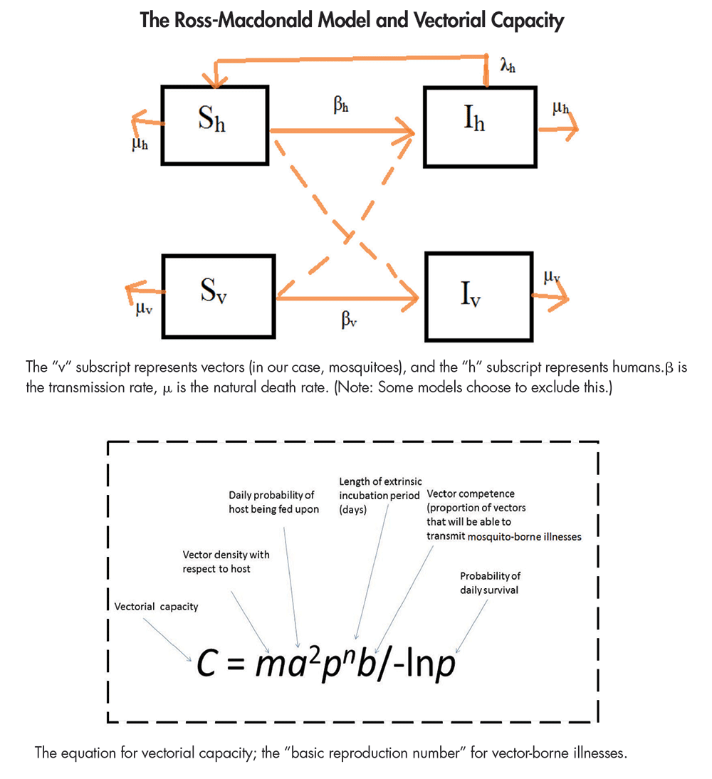
When dealing with diseases such as dengue, chikungunya, and Zika, there is an added layer of complexity to the compartment models of the disease: the need to model the vector (mosquito) population. To track the susceptible and infected mosquito populations, we have to add at least two additional “compartments” for mosquitoes. Overall, the number of boxes that we have to track for the state of all individuals in the system doubles. This leap in theoretical framework came in the 1950s, and can be attributed mostly to the work of George Macdonald, who published The Epidemiology of Malaria while at Oxford.
The Ross-Macdonald model has since become the most accepted compartment model for mosquito-borne diseases and allows us to predict the basic reproduction rate of malaria mathematically. It was from the Ross-Macdonald model that the basic equations for vectorial capacity was developed.
Adding these compartments requires prior knowledge of the mosquito life cycle. This requires us to make certain assumptions and ignore real-life complexities. In addition to human population structure, we ignore the fact that mosquitoes may prefer some people over others. We ignore the reality that mosquito populations are often weather-dependent and seasonal. Last, but certainly not least, we are not able to model intricacies of the diseases themselves. For example, dengue has four different serotypes whose interactions cannot be modeled with a simplistic, Ross-based model.
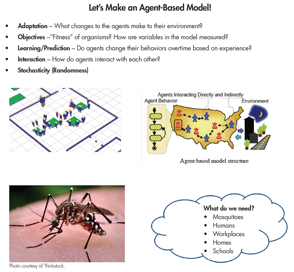
The latest and greatest trend in mathematical modeling is the agent-based model (ABM), which is often viewed as predictively more powerful than the compartment model. An ABM is a powerful simulation modeling technique that has seen a number of applications in recent years. In an ABM, a system is modeled as a collection of autonomous decision-making entities called agents. Each agent assesses its situation individually and makes decisions on the basis of a set of rules.
This is a clear departure from compartment models; with ABMs, we model individuals. Agents may execute various behaviors appropriate for the systems they represent—for example, going to school, going to work, and socializing. At the most basic level, an ABM consists of a system of agents and the relationships between them. Put simply, we can create virtual environments generated from data and run disease simulations to study the dynamics.
Our ABM is generally a bit more complicated with the need for modeling the mosquito population. In an ABM, simulated mosquitoes are not restricted to compartments, and are free to move in a “model domain” as they alternate between seeking blood meals and oviposition sites while interacting with their immediate environments. The simulated mosquito population can be visualized much like the actual population: as a cloud of points in the model domain representing individuals at their locations at particular times.
The previously discussed compartmental models would lump mosquitoes into an aggregated number of individuals and lose the spatial information. In the ABM, relevant characteristics are tracked for individual mosquitoes, including location, age, infection and blood meal status, and size. Each of these attributes is updated for each model time step as the mosquitoes move randomly throughout the model domain in search of oviposition habitat or blood meals, depending on their stage in the life cycle.
ABMs come with many benefits, including the ability to capture emergent phenomena. Systems are described in a “natural way,” which leads to wider acceptance of the modeling approach. Models are more flexible and can easily be adapted to new constraints. Agent-based modeling can be applied if you would like to explore the natural representation as consisting of interacting agents, the problem can be described in terms of individual behaviors of participants, and the behavior of participants can be defined directly.
An agent is defined as an individual or collective entity that is autonomous, with a capability to adapt and modify its behaviors. It also allows us to study how agents adapt and change their behavior during the simulation. Agent-based modeling gives us insight into the relationships among participants of the system, and can even demonstrate results of adaptive behavior. With all of these considerations, agent-based modeling becomes one of the most dominant mechanisms for modeling mosquito-borne illnesses like Zika.
By viewing epidemics as a dynamic process, we can also evaluate potential control measures. Experts have suggested applying larvicide, organizing neighborhood cleanup campaigns, and even throwing out old tires (the tires serve as a breeding ground for mosquitoes) to stop the spread of Zika.
As an alternative to methods that depend on unreliable case data, a research team from the University of Notre Dame developed and applied a new method that “leverages highly spatially resolved data about drivers of Zika transmission to project that 1.1 (1.0–1.9) million infections in childbearing women and 64.2 (53.6–108.1) million infections across all demographic groups could occur before the first wave of the epidemic concludes” (Perkins).
This projection is largely consistent with annual, region-wide estimates of 53.8 (40.0–71.8) million infections by dengue virus, which has many similarities to Zika. This projection is also consistent with state-level data from Brazil on confirmed, Zika-associated microcephaly cases, and it suggests that the current epidemic has the potential to have a negative impact on tens of thousands of pregnancies.
The model was based on the Ross-Macdonald model, and the R0 was also a function of temperature, mosquito distribution (“occurrence”) probability, and the purchasing power of a given country (an economic indicator).
The estimates of the R0 were shaped by three environmental variables: temperature, mosquito (Ae. aegypti species) occurrence probability, and economic index. With respect to temperature, peak values of the R0 were obtained at around 30°C. Differences in the R0 attributable to differences in the economic index also increased steeply as lower economic index values were approached.
With new, emerging diseases, it is also common to analyze the attack rate of the epidemic, which is used to convey the number of victims from a given diseases. In a typical SIR model, there is a one-to-one relationship between the R0 and final epidemic size. Overall, projected values of the reproduction number were consistent with published estimates of the R0 for chikungunya.
Perhaps this similarity with other mosquito-borne illnesses (dengue and chikungunya) would allow for analyses and control methods of those diseases to be applied to Zika. Overall, projections from this model provide feedback on the magnitude of the epidemic and can allow for better outbreak response. The research done so far on Zika’s “epidemic burnout” could serve as a reminder about the “transient nature of epidemics” (Perkins). Still, for those for whom the option is available, postponement of pregnancy until after the first wave of the epidemic passes could be the best strategy for minimizing risk.
The ability to make predictions about epidemics is one of the major strengths of mathematical approaches. Using models, we test control strategies without interfering with the real world. We can, therefore, compare treatments and interventions before putting them into practice. Thanks to Ross and his successors, we no longer have to tip over the water tank to find out what effect it might have.
Further Reading
Bollet, Alfred Jay. 2004. Plagues and Poxes: The Impact of Human History on Epidemic Disease, Vol. 2. New York: Demo Publications.
Chowell, G., C. Castillo-Chavez, P.W. Fenimore, C.M. Kribs-Zaleta, L. Arriola, J.M. Hyman. 2004. Model parameters and outbreak control. Emerging Infectious Disease Journal 28 March 2016].
Day, Troy, A. Park, N. Madras, A. Gumel, J. Wu. 2006. When Is Quarantine a Useful Control Strategy for Emerging Infectious Diseases? American Journal of Epidemiology 163 (5): 479–485. doi: 10.1093/aje/kwj05.
Harling, Guy. 2016. Ebola epidemiology roundup #6. Constrained Optimization.
Heesterbeek, J.A.P., and M.G. Roberts. 2015. How Mathematical Epidemiology Became a Field of Biology: A Commentary on Anderson and May (1981), “The Population Dynamics of Microparasites and Their Invertebrate Hosts.” Philosophical Transactions of the Royal Society B: Biological Sciences 370.1666: 20140307.
Hurford, Amy. 2016. Ronald Ross’ mosquito theorem. Just Simple Enough: The Art of Mathematical Modelling.
Kukaswadia, Atif. 2016. John Snow: The First Epidemiologist. Public Health Perspectives.
Last, John M. 2002. Epidemic Theory: Herd Immunity. Encyclopedia of Public Health. Encyclopedia.com.
Legrand, J., R.F. Grais, P.Y. Boelle, A.J. Valleron, A. Flahault. 2007. Understanding the dynamics of Ebola epidemics. Epidemiology and Infection 135: 610–621.
Nelson, Kenrad E., and Carolyn Williams. 2014. Infectious Disease Dynamics. Infectious Disease Epidemiology 131–50.
Perkins, T. Alex, Amir S. Siraj, and Corinne Warren Ruktanonchai. 2016. Model-based projections of Zika virus infections in childbearing women in the Americas.
Ross, Ronald. Malaria Site. 25 Feb. 2015. Web. 27 Mar. 2016.
Schwan, Katharina. “Spotlight on Zika Virus: An insect-borne STD?” The disease daily. N.p., 5 Feb. 2014. Web. 27 Mar. 2016.
Smith, David L., et al. Ross, Macdonald, and a Theory for the Dynamics and Control of Mosquito-Transmitted Pathogens. PLOS Pathogens.
About the Author
Abby Smith is currently a master’s student in Statistical Practice at Carnegie Mellon, where she received a BS in Mathematics in May 2016. She hopes to pursue a PhD in the use of statistics to inform health, education, and human rights policy.


