Nolan and Temple Lang (2010) stress the importance of knowledge of information technologies, along with the ability to work with large data sets. Relational databases, first popularized in the 1970s, provide fast and efficient access to terabyte-sized files. These systems use a structured query language (SQL) to specify data operations. Surveys of graduates from statistics programs have noted that familiarity with databases and SQL would have been helpful as they moved to the workforce.

Database systems have been highly optimized and tuned since they were first invented. Connections between general purpose statistics packages such as R and database systems can be facilitated through use of SQL. Table 1 describes key operators for data manipulation in SQL.

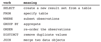
Table 1—Key Operators to Support Data Management and Manipulation in SQL (Structured Query Language)

Use of an SQL interface to large data sets is attractive as it allows the exploration of data sets that would be impractical to analyze using general purpose statistical packages. In this application, much of the heavy lifting and data manipulation is done within the database system, with the results made available within the general purpose statistics package.

The ASA Data Expo 2009 website provides full details regarding how to download the Expo data (1.6 gigabytes compressed, 12 gigabytes uncompressed through 2008), set up a database using SQLite, add indexing, and then access it from within R or RStudio. This is very straightforward to undertake (it took the first author less than two hours to set up using several years of data), though there are some limitations to the capabilities of SQLite.

MySQL (described as the world’s most popular open-source database) and PostgreSQL are more fully featured systems (albeit with somewhat more complex installation and configuration).

The use of SQL within R (or other systems) is straightforward once the database has been created (either locally or remotely). An add-on package (such as RMySQL or RSQLite) must be installed and loaded, then a connection made to a local or remote database. In combination with tools such as R Markdown (which make it easy to provide a template and support code, described in detail in “Five Concrete Reasons Your Students Should Be Learning to Analyze Data in the Reproducible Paradigm”) students can start to tackle more interesting and meatier questions using larger databases set up by their instructors. Instructors wanting to integrate databases into their repertoire may prefer to start with SQLite, then graduate to more sophisticated systems (which can be accessed remotely) using MySQL.

The dplyr package encapsulates and replaces the SQL interface for either system. It also features lazy evaluation, where operations are not undertaken until absolutely necessary.

Another option in dplyr is for the user to directly specify SQL SELECT commands (this is an important topic for statistics majors to see at some point in their programs). For example, the following code would replicate the creation of the data set of counts for the three airports used to create Figure 2 using SQL (as opposed to using the interface within dplyr).

flights <-
dbGetQuery(con, “SELECT Dest, Year, Month, DayOfMonth, DayOfWeek, sum(1) as numFlights FROM ontime WHERE (Dest = 'ALB' OR Dest = 'BDL' OR Dest = 'BTV')
GROUP BY Year, Month, DayOfMonth, Dest”)

In this example, a set of variables is selected (along with a derived variable which sums the number of flights) from the three airports of interest. The results are aggregated by day and destination (at which point they are more manageable). The dbGetQuery() function in the RMySQL package returns a dataframe containing the results from the SQL SELECT call. The SQL syntax is similar, but not identical, to the dplyr syntax.

Is setting up a database too much effort? We think not (and provide further guidance at the aforementioned website). As another option, those willing to explore can undertake similar analyses using the nycflights13 package on CRAN, which includes five dataframes that can be accessed within R (see the previous link for example files).