
Luck and Skill in Tournament Golf

On June 16, 2005, a field of 156 of the finest male golfers in the world played the first round of the 2005 U.S. Open, one of the four “major” annual tournaments in men’s professional golf. The list of entrants included nearly every major tournament player of the past few years, and all of the players were present either by invitation or because of excellent play in previous outings. Most of them were players at or near the top of their game, and had to be considered threats to win or at least place highly in this rich tournament.
With a prize of more than $1 million to the winner, all could be expected to give that initial round their maximum concentration—yet, they played that round with widely varying results: The average score for the day was 75, and the range ran from 67 to 85.
All 156 of these competitors were splendid golfers; 148 were top professionals and the other eight were the best amateurs in the country. Why should their performances vary so much on a single day?
Two reasons present themselves. The first is that while all were splendid golfers, perhaps they were not equally splendid: There was, without doubt, some variation in skill levels. The second is that the entrants benefited unequally from what is commonly referred to as “luck.”
An examination of the sizes and relative importance of these two components of the variation in scores of top tournament golfers is a principal goal of the study discussed here. A secondary and more-speculative aim is to see what implications can be drawn from this narrowly focused and quantitative study about the balance of skill and luck more generally—in other sports and in the social world.
Skill and Luck
“Skill” and “luck” are common terms in everyday language, but the sense in which they are used here requires discussion.
“Luck” is perhaps the simplest of the two: By a player’s luck, we refer to transient variations in a player’s score; that is, variations particular to that player (which do not reflect some common cause that affects all players that day). Luck does not tend to persist from day to day over the four days of the tournament. Luck may be score variations due to bad or good bounces or wind gusts, to chance encounters with obstructions or spectators, to nervous reactions of a moment.
We specifically do not count as luck the good fortune that seems to belong to certain players systematically: Such luck is persistent and properly called skill. By luck, we mean changes in score that would occur for a single player if he or she were to replay the same round under exactly the same
conditions, day after day, without any benefit from the experience.
“Skill” is more difficult to describe, particularly because we mean to emphasize aspects of skill that differ from ordinary understanding. All of the entrants possess skills at the very highest level; it would seem foolish to raise even the slightest doubt that skill is the predominant determinant of success in tournament golf, but a little reflection shows the error of this way of thinking.
Suppose for a moment that the very best golfer in the world could be cloned,and imagine a tournament consisting of 156 exact clones of that golfer. Skill would play no role at all in the outcome of that imaginary tournament—it would be decided entirely by what we call luck. Yet if we were to add a single ordinary mortal to that pool of talent, the situation would change dramatically, and the skill difference of the mortal and the clones would be evident to all.
The point is that the absolute level of skill of the players is unimportant to the result of any tournament. Only variation in the skill levels of all those competing is important; only the relative skills of those competing play a role in the determination of the winner.
Skill in each golfer is the persistent capacity to play at a certain level, a capacity that we will suppose remains unchanged over the four days of the tournament. If a single player were to play the same course under exactly the same conditions repeatedly for many days, then the difference between that player’s average score per round and the similar average for all tournament entrants will be that player’s skill.
Our principal object is the study of the variation in different players’ skills among the entrants and the comparative magnitudes of this variation and the variation in luck for individual players. This relationship will influence the outcome of the tournament. When the skill variation dominates, the more-skillful players will finish near the top consistently. When luck variation dominates, no single player or group of players will win consistently.
Since a tournament extends over four days, we recognize one other sort of variation: the day-to-day variation due to conditions supposed to affect all players equally, such as pin placement, weather condition, or general media stress. We comment later on the possible effect such variation may have on the analysis if it affects only some of the players, such as a weather change in the middle of the day.
A Simple Model
Tournament golf is a very complicated enterprise, so it is surprising that a great deal can be learned from a model that ignores much of the complication. The proposed model is the essence of simplicity:
Player’s score in a round = par for the day + player’s skill + luck.
More formally, the score of the ith player on the jth day of the four day tournament, Xij, can to a reasonable approximation be given as:
Xij = μj + Si + Lij.
Here μj is the par for the day: notionally, if these same players were to play repeatedly exactly the same course under the same conditions, this would be their average score. The skill of the ith player, Si, would be the average difference between that player’s score and the daily par (average of Xij – μj) over a long run of play where the player’s ability remains unchanged.
Note that high scores are not desirable in golf, so a large positive Si corresponds to low skill here. Players with high skill would have negative Si. Lij is the player’s luck in that round, defined as:
Lij = Xij – μjj – Si.
Expressed that way, the relationship is tautological, but it ceases to be so with a few further assumptions: We suppose, most importantly, that the luck and skill are statistically independent—that players at all levels are subject to the same magnitude in variation due to luck, be they average tournament players, the top rung in the tournament, or the below-average. That is, the level of play varies with the skill S, but variation day-to-day is the same for all.
This assumption can be and will be checked against the data later (it passes). The remaining assumptions are that the skills of the players entered—the Si—are distributed independently as a normal distribution with mean 0 (the daily par having been subtracted) and variance σS2, and that the Lij are distributed independently as a normal distribution with mean 0 and variance σL2. The daily pars μj are considered to be four constants, different in each tournament.
The analysis is based upon the recorded player’s scores in a large number of tournaments. We estimate, separately for each tournament, the μj and the variances σS2 and σL2. Note that σS2 is the variance of skills of all entering players, regardless of whether they eventually make the cut.
The interest in this model comes from the ease of interpreting the results from these estimates. For one player in one round, we have:
Xij = μj + Si + Lij.
This, under the model’s assumptions of independence, gives a simple expression for the relative contributions of the two sources of variability for a randomly selected player:
Variance(Xij) = Variance(Si) + Variance(Lij) = σS2 + σL2.
The two variances may differ, but they are weighted equally. However, over a four-day tournament, the luck “averages out” to a degree and the player’s variability in total score—Σj Xij—has a different breakdown:
Σj Xij = Σj μj + 4 Si + Σj Lij.
and
Variance(Σj Xij) = Variance(4 Si) + Variance(Σj Lij) = 16σS2 + 4σL2.
Here, the weight of skill over luck is 4 to 1. We will discuss the implications of these relationships in the light of data collected over more than 20 years.
The Data
The primary data are the results of all four “major” men’s tournaments—the Masters, PGA, and U.S. and British Opens—for all 22 years from 1994 through 2015. In addition, we looked at data for a less-complete set of major women’s tournaments: the Women’s PGA for 10 years (2001–2009 and 2014) and the Women’s Open championships for 10 years (2001–2009 and 2013).
In every case, all golfers who completed the tournament were included—”completed” meaning they were either cut after two full rounds or finished all four rounds. Thus, in the 2005 U.S. Open, 156 golfers completed round 1, but only 154 completed the tournament, the other two dropping after round 1 and before the cut. In every tournament, the daily pars and skill and luck variances were estimated by maximum likelihood.
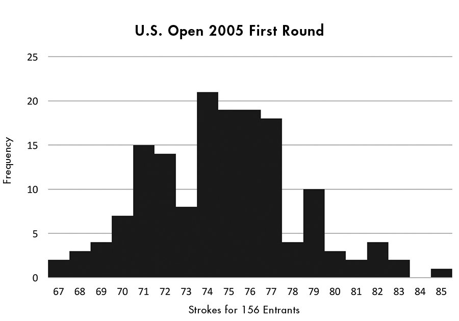
Figure 1. Results of first round of U.S. Open, June 16, 2005.
The estimated skill and luck variances for the 108 tournaments are summarized and displayed in Figure 2.
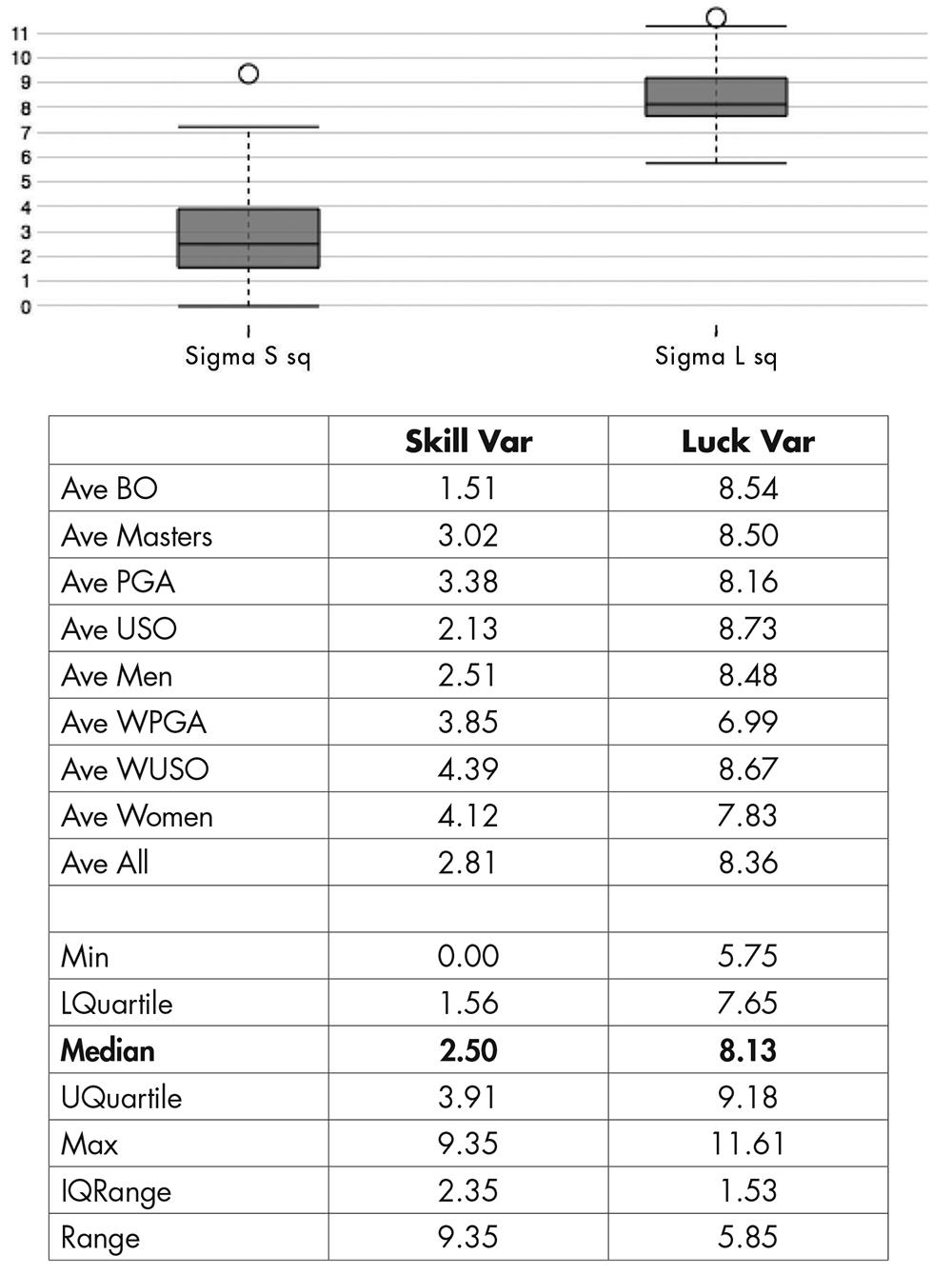
Figure 2. Estimated skill and luck variances for the 108 tournaments,summarized.
The first striking feature is the remarkable lack of variation in the luck variance: In a full 50% of the cases, the estimates fall between 7.65 and 9.18; the median is 8.13 and the mean is 8.36. The luck variance is essentially the same for men, women, and in all tournaments. As shown later, it is also the same from the top golfers down through the bottom quartile.
The second striking feature is how large this variance is: A median variance of 8.13 gives a standard deviation of 2.85, which suggests a luck variation of plus or minus 5.5 strokes a round is not unusual. The irreducible luck component is large and may be expected to have a considerable effect upon outcomes.
What about skill? The situation there is mixed in interesting ways. The smallest skill variance is in the British Open; the largest in the women’s tournaments (both individually and in aggregate). In fact, of the 22 British Opens, two have skill variance estimated to be zero, and three others are nearly as small. We suggest two explanations for this.
The first is that the British Open is typically held on narrow courses bounded by treacherous rough and with numerous hazards that are not familiar on the PGA tour in North America. If we add to that the frequently unfriendly character of the weather on the Scottish coast, the skills perfected on the calmer, manicured courses in America may just be less relevant. The course may not be physically level, but the “playing field” of relevant skills may be unusually so.
The other explanation may be related to weather also: The model we use makes no allowance for changes in conditions during a round that may favor early or late starters. Changes between days are allowed by the model through the par, but not within days, and to the degree this happens, the model would attribute a good part of the change to luck.
We suspect both causes are present there in different years. Indeed, the two Opens with skill variance estimated to be zero (2008 and 2013) have the two largest estimated luck variances in any of the men’s tournaments: 11.05 and 11.27. The model may simply fit the British Open less well.
The larger skill variance for the women’s tournaments seems likely to be tied to differences between the two tours. The women’s tour is much smaller than the men’s, presumably due to being much more poorly compensated, and so it is far more difficult for women to reach a subsistence level on tour. The 2017 purse for the women’s U.S. Open was $5 million, the largest purse of any women’s tournament (the WPGA the same year was $3.5 million), but small compared to the Men’s U.S. Open that year at $12 million.
While all the winners of the women’s tournaments do well (top prizes of $500,000 or so; still much less than the men, who may take over $2 million), the lowest prize among those who made the cut for the 2017 Women’s U.S. Open was less than $7,000, not even close to covering expenses, and those who missed the cut got nothing.
The top players on both tours are superb golfers who can continue to survive, but the middle and lower players on the women’s tour can only remain for a short time unless they meet success. The men have many more tournaments, and richer prizes, and while it is also difficult to survive in that tour, many more enter and only the best of these make it to the majors. The women’s majors draw from a smaller pool, and must draw more deeply.
As mentioned earlier, the variance of total scores over four rounds is 16σS2 + 4σL2, which weights skill over luck by 4 to 1: Skill will outweigh luck if 4 times the skill variance exceeds the luck variance (see Table 1).
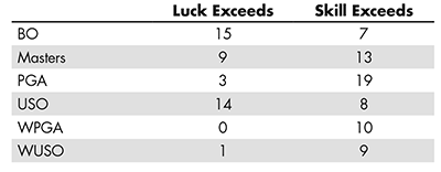
Table 1—Luck vs. Skill
Bear in mind that “skill” here means range of skills among initial entrants, not absolute skill, and that certain types of within-day weather changes (for example, as in some British Opens) that favor early starters will contribute to variation as “luck” for our model.
By running over four days, a golf tournament balances the contributions of skill and luck. Table 2 shows how this goes, “ratio” being = (#rounds) x σS2/σL2.
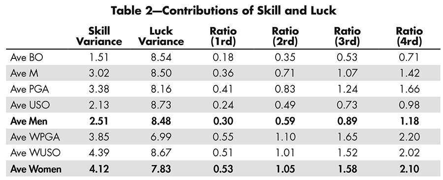
Table 2—Contributions of Skill and Luck
For men’s tournaments, a one-day/one-round plan would have luck variation exceeding skill variation by more than 3 to 1; four days of play moves the balance considerably to slightly on the other side. Clearly, the balance varies: It is much more weighted toward luck for the British Open, as noted earlier (where the effect of weather plays a role, too), and much more toward skill in women’s tournaments. However, since the 1930s, most tournaments have run for 72 holes played over four days. It seems reasonable to speculate that 80 years ago, the skill variation for the men would have been more like that for women today: The number of professional men then was much smaller and the purses much lower.
The need to balance skill and luck requires a tournament to run several days; for the better part of a century, the four-day, 72-hole tournament has served as a convenient compromise.
The Constancy of Luck Variation
Our simple model supposes that luck variation is the same for all players, from the best to those who fail to make the cut. To see if the data support this assumption, we looked at all 66 golfers who entered both the Masters and the PGA in 2005. We ordered them according to their total scores for the two tournaments. Players 1 to 32 made the cut in both tournaments, and players 59 to 66 missed the cut in both; the others (33 to 58) made the cut in one but not the other.
Player #1 was Tiger Woods; he won the Masters and finished third in the PGA that year. Player #2 was Phil Mickelson; he won the PGA and finished ninth in the Masters. For each player, we estimated the standard deviation per round (after subtracting the estimated daily par for each completed round, we estimated the variance for each player for each tournament, pooled these with appropriate weights, and took the square roots). The display shows no pronounced violation of the assumption; the increased scatter for the lower-ranked players reflects the fact that fewer data were available from tournaments where the cut was missed.
A natural question to ask is how likely is the golfer with the highest level of skill to win a tournament? That turns out not to be quite the right question: The chance the most-skillful player will win depends tremendously upon the gap between the top player and the second-most–skillful player, and upon the tightness of the grouping of skills among the others behind the second.
Instead, we looked at the dependence of the probability of winning on the gap between #1 and #2, supposing the players below #2 had an average configuration for a Men’s PGA tournament (see Technical Appendix).
In a small simulation study using the median values for our data of σS2 = 2.50 and σL2 = 8.13, we found that if the top player has an average 1-stroke advantage over #2 (i.e. S1 = S2 – 1), the probability of winning is about 31%; the chance of finishing second is about 16%. If the advantage is increased to an average 2-strokes (S1 = S2 – 2), the chance of winning rises to about 58% and the chance of finishing second is about 16%. To get a feeling of what this means, a one-stroke advantage is quite large at this level of play. Under our model, the expected gap between the top two entrants is only 0.4 strokes, and the top entrant is expected to win 16% of the time.
A two-stroke advantage is almost unheard of. It is said that at his very best, Tiger Woods played an average of about two strokes a round better than the nearest competitor, a level he could not sustain for long.
Regression
This study began in April 1996, initially to answer a simple question. That was the year golfer Greg Norman went into the final round of the Masters with a six-shot lead, but he lost the tournament, ending up five strokes behind Nick Faldo. In the process, he became a symbol of “choking.” The next day’s Chicago Tribune headline stated, “Norman Gags.” Indeed, his descent was steady from the beginning; the top of the leaderboard after the fourth round looked like this:
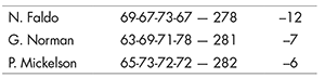
If you were to plot Norman’s four rounds, they show an almost-linear trend for the worse. But was Norman really unusual in his performance? Many others in the same tournament showed a similar (but less-severe) trend. In fact, of the 44 who finished, 33 showed a net trend for the worse and 9 showed a trend for the better. Two golfers showed no trend at all, including the eventual winner, Nick Faldo.
The course did play a bit harder in the later rounds, but correcting for that has little effect; 30 of the 44 still trended for the worse.
We suspected that much of this was simply evidence of the “regression to the mean” phenomenon: If two variables X (a golfer’s score on the first two rounds) and Y (same golfer for the last two rounds) are imperfectly correlated, and an individual is selected on the basis of an extreme value of X, then we should, on average, expect that in standard deviation units, Y should be closer to the population average than is X.
The 44 who finished the 1996 Masters were selected as (roughly) the top half of the entering field of 92, based upon their total score in the first two rounds. We should expect an apparent drop in performance for the second half. This is true even supposing (as we do) that their skill remains intact: If their first-half performance was due in part to good luck, that component could not be expected to continue; they would go from “Good Skill + Good Luck” to “Good Skill + Average Luck.”
The regression phenomenon surely played a role for the field as a whole, but was it enough to account for Norman’s fall from grace? In terms of our simple model, (X, Y) are bivariate normal with means μX = μ1 + μ2 and μY = μ3 + μ4, variances Var (X) = Var (Y) = 4σS2 + 2σL2, and correlation ρXY = 2σS2/(2σS2 + σL2). Given the total score for the first two rounds and assuming “no choking” (so the skill remains the same), the conditional expectation for the last two rounds is then E(Y|X = x) = μY + ρXY(x – μX).
Using the data for the 1996 Masters to give estimates of the means and correlation, we have that for Greg Norman, x = 63 + 69 = 132, so E(Y|X = 132) = 149.7 + 0.459(132 – 147.8) = 142.45, but his actual score for the last two rounds was 71 + 78 = 149, or 6.5 strokes worse than the regression predicted.
Norman lost by 5 strokes; had he only regressed as expected, he would have won. On the other hand, 6.5 strokes is only 1.5 “luck” standard deviations, so the evidence for choking, while quite suggestive, is not absolutely compelling.
An Interesting Contrast
Tournament golf and several other sports balance the effects of skill and luck by adjusting the length of the tournament. NCAA basketball also structures its major tournament (“March Madness”) for such a balance, but they do it in a totally different manner. The basic tournament (after some minor stages to allow a few marginal teams to enter late) involves 64 teams that are thought by the organizers to be the best in the USA. This choice is made very late in the season, when there is a great deal of information on their ability; it is not a random selection.
In a way, their problem is that there is too much information on skill: If 10 experts were to independently each name for whom they thought were the 10 best teams, there would be a considerable overlap. Why is this a problem? Because there are too many teams to allow the same two teams to play multiple times, and in any single game, if two teams play that are at all similar in skill, there is a nontrivial chance the weaker will beat the stronger.
If any two teams in the top half of the 64 were to play a single game, the data suggest the chance of an upset is above 15%. For the top quarter, it is above 30%. The organizers evidently worried that if the structure used random pairings (so, for example, the top two teams might play each other in the first round), there would be a good chance that the best teams would be knocked off early, and fan interest and the credibility of the tournament would suffer. The effect of luck was too strong.
To deal with this, the NCAA divided the field of 64 into four evenly matched divisions of 16 teams each, and in each division, they ranked (“seeded”) the teams in the organizers’ judgment from 1 (best skill) to 16 (lowest skill). They then set up a schedule of play (“the bracket”) that would determine the paired match-ups; each division would produce a winner; these would then be paired for the semifinal matches; and the one final match between the semifinal winners would decide the championship. In the first round in each division, the #1 seed would play #16 seed, #2 seed plays #15, …, and #8 seed plays #9 seed. In the second round, the winner of #1 vs. #16 plays the winner of #8 vs. #9, and so forth.
The goal was to try to limit the chance a top-seeded team would be eliminated early, and this part has been fairly successful: Through 2017, no #16 has ever beaten a #1 since this version of the structure was introduced in 1985 (in 2018, the overall favorite was upset, to everyone’s surprise). On the other hand, the #8 vs. #9 game is even (53% wins for #9). The second round has gone to the #1 seeded team in the division about 85% of the time.
If the plan was to reduce the role of luck in the early rounds of the tournament, it was moderately successful. Over the 26 years from 1985–2010, 80% of those who survived the third round were initially seeded among the top four in their divisions. With random assignment of opponents, we would expect only about 70% of those survivors to initially be among the top four, using past data to estimate the chances of one seed beating another.
The final rounds are another matter altogether: There, the opponents are much more evenly matched (the flip side of what the structure led to in the early rounds), and the role of luck then becomes magnified.
In March Madness, the role of luck was, by design, shifted to the late rounds—and that of skill to the early rounds; a very different balance from golf. To sustain fan interest, the top seeds have a protected status early on, and the result is as predicted: In the 26 years from 1985–2010, the champion was one of the four #1 seeded teams 16 times. The prize went to one of 12 teams seeded among the top three in one of the four divisions 23 times out of 26.
Conclusions and Speculations
It has not escaped our notice that the balance we find between skill and luck in tournament golf may be expected in other sports as well, and in many social practices beyond sports. No sport where luck dominates can be expected to hold the public’s interest: Lotteries are all luck and attract no spectators and, even though the sums involved can cause a stir, there is no consequential interest in who wins beyond the winner’s immediate family and predators eager to help the winner invest.
At the other extreme, no sport where skill is paramount will consistently attract much interest. Chess comes closest, but even there, it is the potential for human error that holds the occasional small crowd. A contest between two computers will not even be watched by other computers. The twin lures of human excellence and uncertainty are what rule. Just as the structure of a golf tournament is presumably intended to generate interest (and consequently income for all involved), so too in baseball, basketball, tennis. In all these situations, the questions would be what is the structure of tournaments and what considerations lie behind what might seem like arbitrary choices?
Similar situations arise in the arts and sciences. Consider the Oscars and the Nobel Prizes. In each case, an award goes to a few from among many highly skilled individuals eligible. In most cases, there is uncertainty beforehand about who will win. The interest in the year’s awards would be minimal if the choices were either predictable with certainty (skill dominates) or made randomly and completely unpredictably (luck dominates). In these examples, the tournament structure is reasonable opaque, leading occasionally to accusations of bias, but the effect—the mixture of skill and luck—is much the same as that of a structured sports tournament.
Further Reading
Mosteller, F., and Youtz, C. 1992. Professional Golf Scores are Poisson on the Final Tournament days. 1992 Proceedings of the Section on Statistics in Sports, 39–51. Washington, DC: American Statistical Association.
Mosteller, F., and Youtz, C. 1993. Where Eagles Fly. CHANCE 6:37–42.
Little, R.J.A. and Rubin., D.B. 1987. Statistical Analysis with Missing Data. New York: John Wiley & Sons.
Technical Appendix
The model employed in the analysis of each tournament is a mixed random effects model with missing data: The scores for the last two rounds of those players who miss the cut are necessarily (by design) not available. By a linguistic quirk, they satisfy the technical definition for “missing completely at random,” since the missingness is determined entirely by the data that are observed, and the model permits, with all available data, writing down and directly maximizing the likelihood, without needing to compensate for possible data-dependent mechanisms leading to missing data.
The fitting uses the EM Algorithm, where the true skills Si are also considered as missing data (Little and Rubin, 1987, pp. 129, 149–151). The iteration converged rapidly except where the skill variance was at or near the boundary value of 0; in those cases, we refit with the boundary value to ensure we had found the maximum.
In all cases, we estimated the estimate’s variances and covariances. We also fit but did not report data for a number of non-major men’s tournaments and the results were much the same as for the majors, especially regarding the constancy of luck variance.
Of course, the model is simplistic; we noted some lack of fit in cases where there were anomalous weather patterns or rain delays, but except for the effect noted (particularly in a few British Opens) where weather augmented the “luck” variation, we were generally satisfied with the fit.
Golf scores are necessarily integer-valued and cannot be strictly normally distributed. Mosteller and Youtz have modeled them as Poisson on a shifted base (1992, 1993), but that too was an approximation, and our data pass the scrutiny of several diagnostic tests for normality (for example, normal probability plots show approximate linearity and a lack of noted skewness, as would be expected with normally distributed data).
Here are some examples of normal probability plots for the first rounds of typical years for four tournaments.
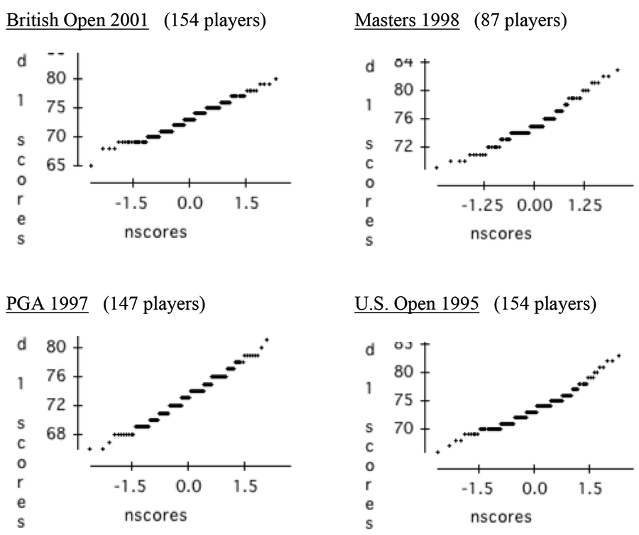
As can be seen, the first round scores for each tournament in the selected years are in straight lines for the most part.
For Greg Norman’s regression equation, we have, in terms of our model, (X, Y) as bivariate normal with means μX = μ1 + μ2 and μY = μ3 + μ4, equal variances Var (X) = Var (Y) = 4σs2 + 2σL2, and covariance Cov(X, Y) = 4σs2, giving the correlation ρXY = 2σs2/(2σs2 + σL2). Given the total score X, the conditional expectation for Y is then E(Y|X = x) = μY + ρXY(x = μX). The data for the 1996 Masters give the maximum likelihood estimates of μ1, μ2, μ3, μ4 as 73.4022, 74.4130, 74.9044, 74.8362, and tthe maximum likelihood estimates of σs2 and σL2 as 3.8794 and 9.1377, so ρXY is 2*3.8794/(2*3.8794 = 9.1377) = 0.4592. Now x = 63 + 69 = 132, so E(Y|X = 132) = 74.9044 + 74.8362 + 0.4592(132 – 73.4022 – 74.4130) = 142.4782.
The small simulation referred to in the section on “The Constancy of Luck Variation” was done in Excel. Recall that according to our simple model, the total score of a player i for four rounds is:
Ti = Σj Xij = Σj μj + 4 Si + Σj Lij.
We created a simulated tournament with 150 entries, first with an ordered column of 280 + 4Si (taking Σj μj = 280 as if par = 70 each round) using an approximation to the expected values of Normal random variables with means 280, and variance 16σs2 = 16*2.5 (16 times the median skill variance from our data). We then added a luck column that was random Normal with mean 0 and variance four times the median luck variance for a single round (since Var(Σj Lij) = 4σL2 = 4*8.13).
If the two columns were added, they would give the results for a simulated four-round tournament (where the “cut” is ignored). This was repeated 250 times and the finishing ranks of the 150 participants computed for each simulated tournament. For the purposes of this study, the highest skill was changed to be the second skill minus 1 and the tournament repeated 250 times; then similarly but with minus 2. This provides the results for both 1- and 2- stroke advantages.
About the Authors
Margaret Stigler has a master’s degree in sports administration from Northwestern University, with a thesis, “Statistics at the Gate,” that examined the attendance trends for baseball parks across the U.S. She now works on data analytics at the Center for Research Libraries in Chicago. She is a more skillful golfer than her father Stephen, who relies more on luck on the golf course.
Stephen Stigler is professor of statistics at the University of Chicago. His latest book is —The Seven Pillars of Statistical Wisdom— (Harvard University Press, 2016). This study is based on collaboration over more than a decade that has not been funded by any government or other agency.


