
Projecting the Draft and NFL Performance of Wide Receiver and Tight End Prospects

Every offseason, the 32 teams in the National Football League add top collegiate talent to their rosters through the NFL Draft. Since the new collective bargaining agreement was signed in 2011, teams have had the opportunity to sign less-costly contracts with newly drafted players, making those players relatively more valuable. Thus, identifying and selecting the highest value player through every round of the draft can clearly benefit teams for the length of the rookie contracts, as seen with the Seattle Seahawks’ selection of Russell Wilson in the third round of the 2012 NFL Draft.
In recent years, NFL analysts and fans have frequently observed that the NFL has evolved into a “quarterback-driven league” or “passing league.” For quarterbacks and their passing offenses to succeed, the teams need talented physical pass-catchers at both the wide receiver and tight end positions. For example, five wide receivers were selected in the first round in 2014, six in 2015, and four in 2016.
The question then arises of how best to evaluate these pass-catching prospects to separate out those who have the highest expected performance. In the past, NFL teams have relied solely on traditional scouting techniques to evaluate talent, but given the success of analytics in other professional sports, some NFL teams have begun to experiment with and use statistics to provide an additional method of evaluating players.
As compared to baseball, which has used analytics extensively for some time now, football features more dependent events, with 22 athletes involved in every play. There is no simple pitcher-versus-hitter one-on-one matchup, since even when considering wide receiver versus cornerback, the quality of the quarterback, offensive line, pass rush, deep safety, and more will all play a role. However, with the increasing quantity of data compiled on the athletes in this sport, statistical methods provide the ability to assess the future performance of various players entering the NFL more accurately than would have been possible in the past.
We have applied statistical thinking to project the future performance of NFL prospects, using data (for players who entered the NFL between 1999 and 2013) that are completely available on public websites, including nflcombineresults.com, Pro Football Reference, and College Football Reference. Here we primarily examine our statistical models for projecting the performance of wide receiver draft prospects (our first paper, “Predicting the Draft and Career Success of Tight Ends in the National Football League,” applied the same techniques to analyze tight ends).
For both pass-catching positions, we have created regression models as well as recursive partitioning decision trees for projecting performance. For our regression models, we use stepwise variable selection to identify the grouping of variables that maximizes the adjusted R2 of the model. Regression models provide insight into the individual effects of each variable, but they are limited to identifying linear relationships. Therefore, we use the decision trees to identify non-linear relationships.
To create our decision tree models, we select the splits in the tree with the highest log-worth:
log-worth = -log10(p-value of F statistic)
Through these two methods, we have identified the grouping of variables that are most predictive of both when a player will be selected in the NFL draft and how the player should be expected to perform in the future.
In our models, we use several different groups of possible predictor variables. These include physical variables, college attended, college performance, and NFL Combine results. These variables can be seen in the sidebar (previous page). The physical variables include measures related to the player’s size. The college-attended variables are dummy variables indicating where the player played college football. The college performance variables measure the players’ college production totals and how large a proportion of that production came in their final college seasons. Finally, the NFL Combine variables measure a player’s speed, athletic ability, and strength.
We also used an array of different outcome variables. For predicting draft results, we simply used draft order as the outcome variable. For predicting future performance, however, we used a group of four outcome variables. These included NFL games started (the number of NFL games a player started in their career), NFL Career Score, NFL Career Score per Game, and NFL Career Score per Year.
We created NFL Career Score as a measure using a player’s NFL receiving statistics:
NFL Career Score = NFL receiving yards + (19.3 * NFL receiving touchdowns)
The 19.3 factor is based on a study by Stuart in 2008 of Pro Football Reference that indicated advancing 19.3 receiving yards, on average, provides the same change in expected points as crossing into the end zone. For the NFL Career Score per Game version, we divide by NFL games played; for the NFL Career Score per Year version, we divide by years pro.
For example, Torry Holt had 13,382 yards and 74 touchdowns over 11 years (173 games played). Thus, Holt had an amazing NFL Career Score of 14,810.2, NFL Career Score per Game of 85.6, and NFL Career Score per Year of 1,346.4. Meanwhile, David Tyree had 650 yards and 4 touchdowns over 6 seasons (83 games). Therefore, Tyree had a more typical performance: NFL Career Score of 727.2, NFL Career Score per Game of 8.8, and NFL Career Score per Year of 121.2.
For the breakdown of NFL Career Scores in the sample, see Figure 1. To identify the predictor variables that are most important for projecting future performance, we find the variables that are prevalent when producing the models that best fit this group of four NFL performance outcome variables.
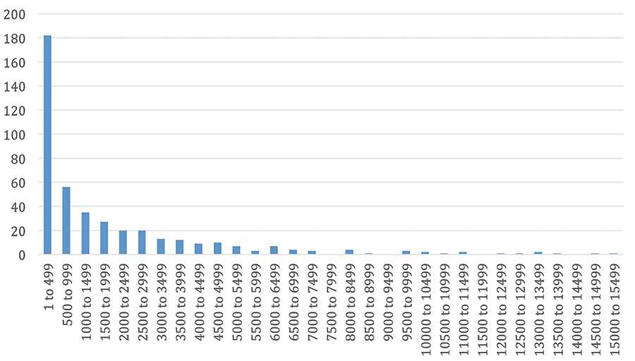
Figure 1. Histogram of non-zero NFL career scores (note: 216 had NFLCS of zero out of a sample of 645 WRs).
We believe that we can capture all of the desirable qualities of a receiver or tight end through these four NFL performance measures. The number of games a player started indicates a player’s talent level, but can also demonstrate leadership and blocking abilities, which are not captured in receiving statistics. NFL Career Score, meanwhile, demonstrates a player’s receiving production and continuity.
NFL Career Score per Game and NFL Career Score per Year also cover receiving production, but without the factor of longevity. NFL Career Score per Game is a variable that only considers on-field receiving performance, while NFL Career Score per Year can also capture whether a player is not always participating in all 16 games (i.e., if affected by injuries or off-field problems resulting in suspensions).
Therefore, through these four variables, we can cover receiving production, longevity, injury/suspension issues, leadership ability, and blocking ability. However, one issue with measuring each of these NFL performance variables is that they are not immediately observable after the draft. Therefore, the data that we used is incomplete for players who are still in the league.
To attempt to account for this, we have required that players be drafted early enough that they have the opportunity to play at least three seasons to be included in our cumulative performance models and at least one season to be included in our average performance models.
In our tight end study, we observed several differences between the predictors of draft results and future performance. For example, we identified bench press as a very significant predictor of draft results, yet it is not significant when predicting future performance, as it was only included in one NFL performance model (and was not significant at the 5% level). Instead, another NFL Combine event, broad jump, is not included in the model predicting draft results, but is included in all NFL performance models (and is 1% significant in all but one).
Along with broad jump, the BCS dummy variable appears in all of the NFL performance models. The BCS dummy variable is included in the draft results model as well, indicating that while level of competition in college does indicate NFL performance, NFL teams are aware of this. In the draft results model, a coefficient of -33.09 indicates that a BCS tight end will, on average, be selected 33 picks (or about one full round) earlier than an otherwise identical non-BCS tight end prospect.
In our analysis, we also discovered that certain other variables (aside from bench press or broad jump) are over- or under-considered when evaluating tight end draft prospects. College receiving statistics, such as yards per reception, receptions, and yards, were under-considered, while a tight end’s 40-yard dash time was over-considered.
This suggests that NFL teams should increase their focus on a tight end’s receiving production in college and pay somewhat less attention to the player’s pure speed.
In our wide receiver study, we identified a large grouping of variables that are predictive of draft results. From this large group, four variables are significant at the 1% level: SEC dummy variable, ACC dummy variable, 40-yard dash, and final year college yards percentage. This indicates that receivers selected the earliest in the NFL Draft tend to come from colleges in either the SEC or ACC, have great straight-line speed, and have a breakout season in their final year in college.
Despite the fact that 14 predictor variables appear in the draft results regression model, none of these are physical variables (height, weight, and BMI). This is a surprising finding, given the fact that many of the elite receivers in the modern NFL, such as Calvin Johnson, Dez Bryant, Brandon Marshall, and Demaryius Thomas, tend to be bigger and taller. Notably, of the five receivers with the best NFL Career Score per Year averages since 1999, four are at least 6 feet and 3 inches tall, with the one exception of 6-foot-1 Torry Holt.
While we didn’t find attention paid to physical variables in predicting draft results, these variables show significance in the models for NFL performance. Specifically, BMI, college yards per reception, college touchdowns, and the ACC dummy variable were the four most-significant predictors (at the 0.1% level) in the NFL games-started regression model. These variables were also among the most significant in the partition tree. Meanwhile, final year college yards percentage and vertical are also significant(1%) in the regression model.
Overall, these results indicate that some of the most significant variables in predicting the draft also are relevant when predicting NFL starts, although there are some differences (in addition to the presence of BMI).
First, vertical replaces the 40-yard dash as the most significant NFL Combine measure, indicating a receiver’s jumping ability is more important than pure speed for becoming an NFL starter. Also, college touchdowns and yards per reception are very significant, indicating that NFL teams should place more emphasis on college production.
It seems logical that wide receivers who are able to find open space in the red zone (with less field remaining ahead) and score touchdowns in college will be more likely to find open space in the NFL despite the faster defenders, particularly when they played in one of the most competitive collegiate conferences (in addition to the extreme significance of the ACC dummy, we find that the SEC, Big 10, and BCS dummies are all 5% significant).
When considering the models for predicting NFL Career Score, we find a similar group of significant variables. The most significant in both the regression and partition models is college touchdowns, again significant at the 0.01% level in the regression. Other variables significant at the 1% level in the regression include BMI, the ACC dummy variable, the BCS dummy variable, 40-yard dash, college yards per reception, and final year college yards percentage, while vertical is significant at the 5% level.
The ACC dummy variable, college performance measures, and vertical are also prominent in the partition tree (accounting for the first three levels of splits), as seen in Figure 2. The group of variables significant in the models predicting NFL Career Score is similar to the group used for predicting games started, but adds the 40-yard dash. The significance of the 40-yard dash in this model indicates that speed may not earn a receiver a starting job, but will help him produce receiving statistics.
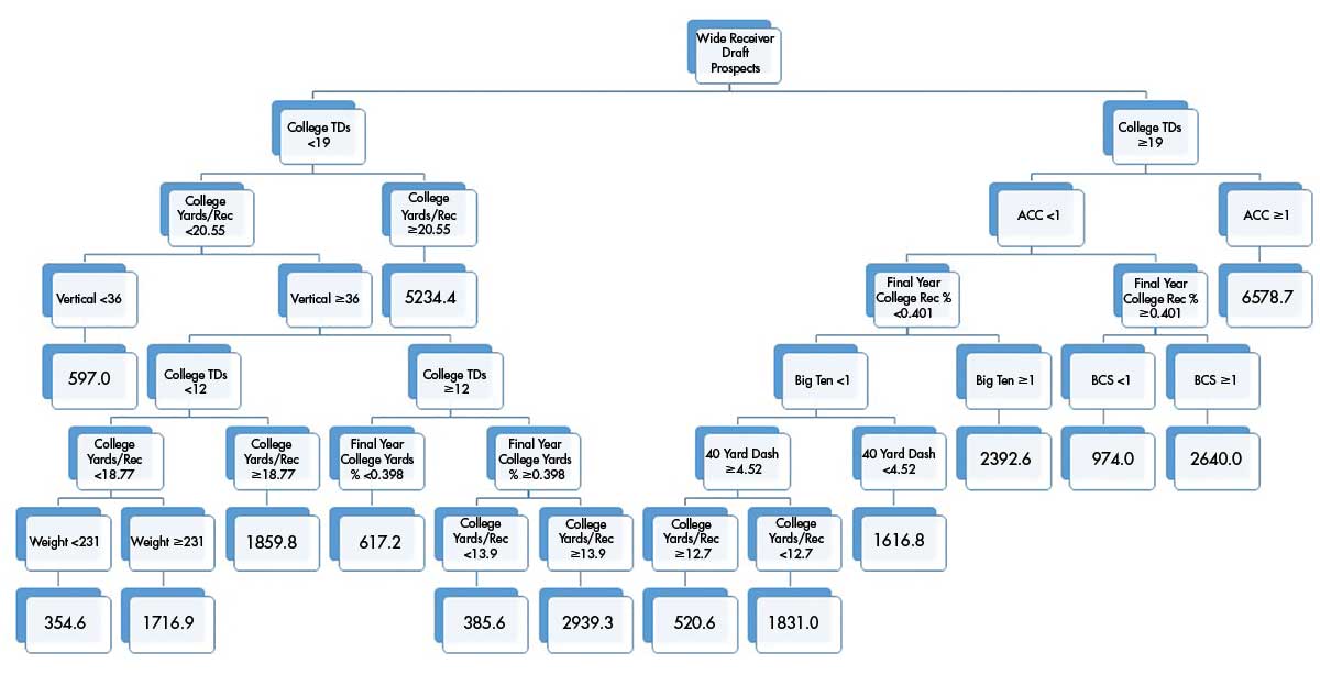
Figure 2. NFL Career Score partition model for wide receiver draft prospects.
The recursive partitioning tree in Figure 2 indicates a predicted NFL Career Score for a wide receiver draft prospect based on the observed value for several variables. Consider Braylon Edwards: He had 39 touchdowns for the University of Michigan, was not in the ACC, had 38.5% of his college receptions as a senior (less than 40.1%), and was in the Big 10.
Therefore, this tree predicted Braylon Edwards to have an NFL Career Score of 2,392.6. Meanwhile, DeAndre Hopkins had 27 touchdowns at Clemson University and, thus, was in the ACC, so this tree predicts Hopkins will have an NFL Career Score of 6,578.7. This is a relatively high NFL Career Score, comparable to those achieved by Edwards (who outperformed the 2,392.6 tree prediction), Santonio Holmes, and Brandon Lloyd.
For the NFL Career Score per Game regression model, size is very significant to prediction of average performance. All three size variables are significant at the 5% level: height, weight, and BMI.
The SEC dummy variable, ACC dummy variable, 40-yard dash, college touchdowns, and final year college yards percentage are all significant at the 1% level, while the BCS dummy is significant at the 5% level. Yet again, the player’s college touchdown total is the most significant predictor of the NFL performance measure (at the 0.01% level).
Additionally, the partition model continues to demonstrate the significance of both college yards per reception and college touchdowns. These models continue to express the significance of college receiving statistics, particularly touchdowns, in projecting wide receiver NFL performance.
The models for NFL Career Score per Year show very similar results to those of NFL Career Score per Game, which is unsurprising since both measure average performance.
Overall, it seems that when evaluating wide receiver draft prospects, college performance, especially touchdowns, stands out as the most prevalent predictor group. However, size and strength (through weight and BMI), speed and jumping ability (through 40-yard dash and vertical), and college attended (specifically ACC and SEC) also show significance.
When comparing these significant variables to those found to best predict draft results, we see similarities in 40-yard dash and the ACC dummy variable, but also several differences. It appears that when evaluating wide receiver NFL Draft prospects, NFL teams should give greater consideration to the players’ college (particularly touchdown) production, jumping ability, and size, since these correlate best with success in the league, as seen in Figure 3.
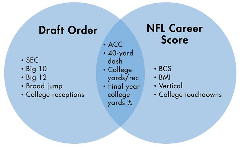
Figure 3. Draft order vs. NFL Career Score: selected variables significant at 5% level in wide receiver regression models.
With these models, we now have the capability to project the future performance of any wide receiver or tight end prospect, so we have applied these models to the 2015 NFL Draft class. Here are our projections for the 2015 wide receiver class.
For the second straight year, a strong wide receiver class entered the 2015 NFL Draft. Six receivers were selected in the first round, including three within the first 14 picks. When analyzing the six first-round picks (Amari Cooper to the Raiders at pick 4, Kevin White to the Bears at pick 7, Devante Parker to the Dolphins at pick 14, Nelson Agholor to the Eagles at pick 20, Breshad Perriman to the Ravens at pick 26, and Phillip Dorsett to the Colts at pick 29), all have high projections from our models. Although all were evaluated highly, Cooper is projected to be the best of these six, while Agholor is the projected as the lowest among these six.
Our model also identifies several non-first-round wide receivers from this class who are projected to succeed in the NFL. These include Devin Smith (to the Jets in round 2), Dorial Green-Beckham (to the Titans in round 2), Tyler Lockett (to the Seahawks in round 3), Chris Conley (to the Chiefs in round 3), Sammie Coates (to the Steelers in round 3), DeAndre Smelter (to the 49ers in round 4), Rashad Greene (to the Jaguars in round 5), and Titus Davis (to the Chargers as an undrafted free agent).
It will be interesting to see how these players perform. The non-first-round wide receivers the model projected to perform well in 2014 (Davante Adams, Jordan Matthews, Donte Moncrief, and Martavis Bryant) all have had impressive starts to their careers.
One other interesting note is the projection for Devin Funchess. The Carolina Panthers selected Funchess, a wide receiver/tight end from the University of Michigan, in round 2 of the 2015 NFL Draft. Funchess projects very badly as a wide receiver, according to our model. This is due to the fact that he ran a 4.70 40-yard dash, several tenths of a second slower than the other top receivers. However, when projected as a tight end, a position at which a 4.70 is better than average, Funchess projects near the top of the class. While the Panthers have primarily used Funchess as a wide receiver, it will be worth seeing if his role changes over time.
The use of analytics continues to rise in all areas of sports, although football is behind many of the others, particularly baseball, of course. While there is far more interaction of players on a football field than on the baseball diamond, our analysis shows that statistical methods are able to isolate an individual player’s potential future performance, and thus likely his contribution to his team.
Our statistical approach can be applied to any position in football, or in any other sport, to create similar models and projections. In another upcoming paper, we have applied this type of analysis to free agent wide receivers and tight ends, while adding NFL performance to date as an additional group of possible predictor variables.
As the teams collect more data over time, the NFL may eventually match the use of analytics found in other major sports leagues. NFL teams will then be able to create models with even larger sets of possible predictor variables, which, in turn, will allow for creating even more-precise predictions of players’ future performance.
We believe that this analysis is also effective in prediction of value (performance per cost), and can be used by teams to optimize player evaluation relative to the salary cap. We include this approach in our published tight end paper and the pending free agent paper.
Further Reading
Hyde, Dave. 2015. How analytics rate TE draft class (Walford? Well…). Sun Sentinel.
Jensen, S.T., and Mulholland, J. 2014. Predicting the draft and career success of tight ends in the National Football League. Journal of Quantitative Analysis in Sports 10(4): 381–396.
Stuart, C. 2008. The final value of a passing touchdown. Pro Football Reference Blog.
About the Authors
Shane T. Jensen, who writes “A Statistician Reads the Sports Pages,” is an associate professor of Statistics in the Wharton School at the University of Pennsylvania, where he has been teaching since completing his PhD at Harvard University in 2004. Jensen has published more than 40 academic papers in statistical methodology for a variety of applied areas, including molecular biology, psychology, and sports. He maintains an active research program in developing sophisticated statistical models for the evaluation of player performance in baseball and hockey.
Jason Mulholland recently completed his undergraduate degree at the Wharton School at the University of Pennsylvania, where he majored in Statistics and Finance. He started conducting statistical research while at Wharton, focused on football, and is now working in finance for the New York Jets.
On Figure 2 if the TDs > 19 and you floow the tree down the left most branch is the last decision split correct. It shows that you get a higher score for having the lower College Yards/Rec numbers. The other places where you check that variable the higher Yards/Rec gets the higher score. Why is this one reversed?