
Modeling Statistical Thinking

In high school, students start to encounter the broader world and prepare for roles as citizens and scholars, teammates, and breadwinners. This makes high school a natural place to help students develop the skills and attitudes to move beyond their individual experiences and toward describing and understanding wider patterns.
The movement from the individual and contingent to the general is, I submit, at the heart of statistical thinking. “Why didn’t you hand in your homework?” is a question about the singular. “The dog ate it” or “My alarm clock didn’t ring” are merely anecdotes—accounts of a singular event. In contrast, a statistically thoughtful question is, “Some students hand in their homework, others don’t. What explains this variation?”
How can educators help students think statistically? There are many possible approaches. The most widespread involves probability; simple descriptions of center, spread, and difference; more-nuanced descriptions with confidence intervals; and testing a null hypothesis.
I advocate another approach: constructing models and putting different models in competition with one another. This article sketches out what I mean by constructing models and tries to demonstrate that techniques, notation, and technology that can support statistical thinking are accessible to a mainstream student.
As a motivating example, consider the relationship between health and lifestyle variables, such as those in a dataset HealthData constructed by reformatting data on n=4048 people surveyed by the U.S. National Center for Health Statistics and made available via the NHANES package in R. Table 1 shows 10 cases out of the 4,048.
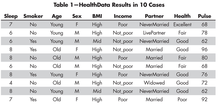
Table 1—HealthData Results in 10 Cases
As in my teaching, calculations and graphics are made with R and the mosaic package for R, which provides easy-to-use facilities for randomization and iteration, and systematically uses the R modeling notation for descriptive statistics, graphics (via the lattice package), and modeling (via the stats package).
To illustrate, consider these few mosaic expressions in R that display the heart-pulse rate of the survey subjects and the association of pulse with other variables.

Note that the same structure is used for all commands, whether they perform a statistical calculation (mean(), sd()) or generate a graphic (bwplot(), shown in Figure 1).

Figure 1. The distribution of pulse for different levels of health
The formula notation, e.g., sleep ~ health, can be interpreted as “sleep as a function of health,” “sleep broken down by health,” or “sleep modeled by health.” The same formula notation is used for statistical models:
![]()
or, with two explanatory variables, plotted out in Figure 2,

Figure 2. A model of pulse using both health and smoker as explanatory variables.

Modeling Framework
As with any statistical method, modeling involves both a conceptual framework and a technical apparatus. In a conventional introduction to statistics, the conceptual framework includes ideas such as the sampling distribution and standard errors; the technical apparatus is made up of items like t-statistics and tabulated probability densities.
One conceptual framework for statistical modeling is this:
- A model can be described as a mechanism for making predictions of future outcomes. The output of a model is the quantity or quality to be predicted. The model’s prediction is based on other variables that are known. The outcome variable is called the response variable. The variables that serve as inputs are called explanatory variables. (On occasion, it is useful to construct models without any inputs; just an output.)
- Models are designed by identifying a response variable and selecting explanatory variables that you believe may contribute to or account for the variation in the response.
- Data are used to specify details of the model; that is, exactly how the selected explanatory variables are related to the response. The term training data is used to identify data used to specify the model; the process is called “training” or “fitting” the model.
- You can evaluate a model by comparing the model’s predictions to the actual outcome: the value of the response variable. For the comparison, you obtain testing data; that is, new data from the same setting as the training data. (In the literature, this is called cross-validation.)
- Models that make more accurate predictions are preferred.
The technical apparatus for a simple form of modeling involves groupwise models and prediction error.
Groupwise Models
For the sake of simplicity, start with models based on means and proportions. Call these groupwise models. For these simple models, only categorical variables can be used as inputs; quantitative variables would have to be converted to categorical before being used. The explanatory variables selected for the model determine which group a case falls into; the model output is the same for all the members of a group, but may be different from one group to another.
As an example, consider a topic that high-school students know about: sleep. A statistical question is, “Some people sleep more than others. What accounts for the variation?” Students will have their opinions. They can be taught to represent these opinions in a mathematical way—as a model. They can also be taught to weigh their opinions against information such as HealthData.
In the simple groupwise modeling framework, constructing a model consists of selecting explanatory grouping variables that account for sleep and finding how the Sleep depends on those variables. Student A might say that the two groups defined by Smoker are important. Student B might claim that Sex and Age are the important factors, giving four groups. Other students will have other ideas, but we can start with these two.
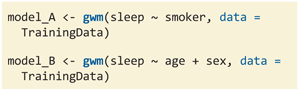
In the “formula” notation in R, the two groupwise models are written with the response on the left side and the grouping variables on the right side.
Student A: sleep ~ smoker
Student B: sleep ~ age + smoker
These model formulas will be fit to training data. The models produced will be:

Used by itself, as in model A, the smoker variable divides the cases into two groups. The two explanatory variables used in model B—age and sex—define four distinct groups. Each group is associated with a specific model value: a number. Here, those numbers are the mean sleep time reported by the people who fall into the respective groups.
Cross-validation and Prediction Error
To fit the models, one first takes a random sample of the data for training the models. I suggest that students use a training sample of, say 10% to 30% of the cases. With n=4,048, the training data might have 1,000 cases.
![]()
The model-fitting process is a matter of calculating groupwise means, and can be accomplished with the mosaic command mean() or, more conveniently for later evaluation, with mosaic’s gwm() function.
Create as many student models as the students come up with. Some students may propose that sleep doesn’t depend on any of the other variables; that there is only one grand group when it comes to sleep. This could be called the “know nothing” model, but it’s traditional to call it the null.
![]()
The 1 in the model can be read as “all in one group.”
Which of these models performs best? One way to quantify the quality of a model’s predictions is the mean square prediction error (MSPE), which is the average across many cases of the square of the difference between the model’s output for that case and the actual outcome of the case. Again, for simplicity, the entire data set HealthData will be used for testing, but it would not be difficult to construct testing data that does not include the training data.
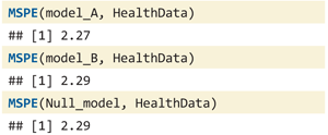
The MSPE measures an error, so a smaller value is better. MSPE would be zero if the model made a perfect prediction. Based on the MSPE, there is not much reason to prefer one model to another.
Model B is no better than the null model. Model A is only slightly better. Conclusion: Neither model explains the variation in sleep.
In many settings, multiple models will perform well. This indicates that each has something to say about the response. As such, the well-performing models can be a seed for generating new hypotheses and continuing the process of investigation.
Traditionally, of course, one uses the entire data set for fitting, not just a sample. But dividing into training and testing data leads to a dramatic simplification in interpretation. When using the same data for training and testing, every model with any explanatory variables will perform better than the Null. Consequently, one has to invoke sampling variation under the Null to reject weak models.
With cross-validation, the whole apparatus of significance can be avoided, including concepts such as degrees of freedom, t– and F-statistics, sampling distributions under the Null hypothesis, etc.
Indeed, a cross-validated model can perform worse than the null; for instance:

Groupwise models can also be constructed for categorical response variables. The output is then a group proportion, which can be interpreted as a probability of having a particular level from among the response variable’s categories. Measurement of the model errors can still be done with MPSE (which, for categorical responses, is a rough approximation to the negative of the log-likelihood).
Groupwise models are not intended to supplement the professional’s toolkit, but they do provide quick access to modeling. As understanding is gained with groupwise models, regression models (e.g., lm() and glm() in R) can be introduced as a replacement and, for starters, used with MSPE(). Regression models require some additional training to understand how to interpret the model co-efficients. The point of using groupwise models here, in a high-school setting, is merely to start things off with minimum conceptual complication.
Other Statistical Topics
The simple groupwise-model/cross-validation approach described in the previous section is intended to support starting the development of statistical reasoning. It is an honest approach that illustrates some important points:
- Hypotheses about relationships among variables can be tested against data.
- Multiple variables can be included in a relationship.
- Patterns can appear accidentally in a sample of data that don’t generalize to a larger population; be careful about over-generalizing (aka “over-fitting”) from the few to the many.
There are additional statistical topics that could be treated using groupwise models and cross-validation. For instance, confidence intervals on the groupwise model values can be generated by either normal theory or randomization. The mosaic package has a particularly nice way to generate standard errors or confidence intervals or p-values using resampling.
Confounding and covariation are tremendously important ideas for statistical thinking. Modeling in general, and linear and logistic models in particular, provides a solid basis for understanding covariation and dealing with it. Conventional, non-modeling approaches to introductory statistics based on sample statistics and hypothesis tests typically make little or no mention of confounding and covariance, other than to warn about “lurking variables.” This leaves the student without examples that highlight what can and should be done in the face of confounding.
Many will regard the cross-validation technique as wasteful of data. Why not use all the data when calculating a sample statistic or fitting a model? Indeed, this issue largely drove the development of the mainstream techniques found in introductory statistics: how to estimate sampling variation without having multiple samples.
Of course, a more-efficient use of data is better …all other things being the same. But they are not the same. For one, contemporary uses of data often involve large data sets (thousands to millions of cases), rather than the traditional handful of cases found in introductory statistics texts. In large data sets, efficiency is of marginal benefit (until you reach the point where the number of variables is also large). More important, in the context of teaching statistical thinking to students first encountering it, the efficient methods come with a burden to learn technicalities that don’t illuminate statistical thinking.
For instance, when the sample size (or, more precisely, the residual degrees of freedom) is 30 or more, there is essentially no difference between the t and normal distributions. When the sample size is greater than, say, 10, there is little practical difference. Why should students starting out in statistics be made to study distinctions with little difference, when their time and energy could be used for exploring confounding and covariation, which, in many settings, have a much larger influence on conclusions than the choice between t and z?
Reflection
In reflecting on the theme of this month’s issue—”Nurturing Statistical Thinking Before College”—it becomes clear that, for many statistical educators, the meaning of “statistical thinking” can traced back to David Moore’s 1990 list of core elements:
1. The omnipresence of variation in processes
2. The need for data about processes
3. The design of data production with variation in mind
4. The quantification of variation
5. The explanation of variation
Later authors have expanded item 5 somewhat to “the measuring and modeling of variability” and using statistical models to “express knowledge and uncertainty.”
A few additional core elements have been proposed:
6. The use of the scientific method in approaching issues and problems
7. [Recognizing that] all work occurs in a system of interconnected processes
8. Analyzing statistical methods to determine how well they are likely to perform
A claim can be made that conventional approaches to introductory statistics cover some of the core elements (e.g., items 1, 2, 4, and, to some extent, 3). The modeling approach does this, but is unique, I think, in contributing to 5, 6, and 7, and more deeply to 3. Modeling, with its recognition that multiple explanatory variables can contribute to a response, is in touch with the complexity recognized by 7 and how that complexity plays out in explaining variation (5).
Although sound arguments are made for embedding statistics in a decision-theoretic framework, many practicing statisticians and statistical educators believe that statistical thinking should fit within the framework of scientific method. The Oxford English Dictionary captures much of the character of scientific method in this definition: “A method or procedure that has characterized natural science since the 17th century, consisting in systematic observation, measurement, and experiment, and the formulation, testing, and modification of hypotheses.” A modeling approach enables students to formulate hypotheses by choosing explanatory variables, to evaluate hypotheses and compare them to competitors, and to generate new hypotheses by considering and modifying others.
It’s hard to see much of this in the conventional approach. The null hypothesis seen by students is rarely of interest itself. Without embracing multiple explanatory variables, tests such as t– or one-way ANOVA hardly suggest a way to modify previous hypotheses.
As for item 8 (the use of statistics to examine the performance of statistical methods), neither the conventional approach nor modeling directly provides much insight. However, simulation and randomization methods do. These are quite compatible with a modeling approach.
For groupwise models, an understanding of the fitting process is accessible to high-school students. Cross-validation and MSPE are similarly accessible concepts. R, RStudio, and mosaic enable the student to get far with just three command templates:
Sampling from a data set: Training <- sample(__WholeData__, size = ____)
Applying a formula to data:__operation__( __formula__, data=_____), where the operation is selected from mean(), sd(), lm(), gwm(), etc.
Reporting on a model:__report_type__( __model__), where the report type can be MSPE() or, for regression models, plotModel(), anova(), rsquared(), summary() for a regression table, etc.
Everything appears to be in place to adopt an approach to statistical and scientific thinking organized around modeling, except, perhaps, instructor development.
Further Reading
Chance, Beth L. 2009. Components of statistical thinking and implications for instruction and assessment. Journal of Statistics Education 10(3).
Cumming, Geoff. 2015. Intro Statistics 9: Dance of the p-values.
Kaplan, Daniel. 2011. Statistical modeling: A fresh approach. Project MOSAIC Books.
Kaplan, D., N.J. Horton, and R. Pruim. 2015. Randomization-based inference using the Mosaic package.
About the Author
Daniel (Danny) Kaplan is DeWitt Wallace Professor at Macalester College. He teaches statistics, mathematics, and computation; serves as principal investigator on the National Science Foundation-supported Project MOSAIC (NSF DUE-0920350); and co-authored the mosaic package in R.

In Taking a Chance in the Classroom, column editors Dalene Stangl and Mine Çetinkaya-Rundel focus on pedagogical approaches to communicating the fundamental ideas of statistical thinking in a classroom using data sets from CHANCE and elsewhere.


