
Influences of Reproducible Reporting on Work Flow
Reproducible Reports
The aspect of reproducible research that has most influenced my own work is the reproducible (or dynamic) report, where a report is a research product such as a journal article, a conference talk, or a progress report for the research team. In a reproducible report, narrative and code are written in explicitly linked scripts. Changes made in the narrative or code in one part of the work cascade through the other parts, generating a fully updated version of the report.
Three books have significantly influenced how I use R reproducibly: Dynamic Documents with R and knitr, Reproducible Research with R and RStudio, and Implementing Reproducible Research, all in the R Series by CRC Press.
In general, Xie focuses on the dynamic document; Gandrud on the reproducible project; and Stodden, Leisch, & Peng (eds.) on all of the above (tools and practices), plus larger issues such as intellectual property, open science practice, large-scale projects, and reproducible publishing. Taken together, these books provide sufficient breadth to address most beginners’ needs and sufficient depth to afford new insights to experienced practitioners.
Dynamic Documents with R and knitr
Yihui Xie

Paperback: 216 Pages
Year: 2013
Publisher: Chapman and Hall/CRC
ISBN: 9781482203530
Each book acknowledges the roughly 30-year history of reproducible research and the debt the community owes to innovators such as Donald Knuth, Jon Claerbot, and others. Still, I credit two recently developed software environments—Yihui Xie’s knitr package and the RStudio IDE—with making dynamic documents easy to create and maintain. (Jeff Leek adds IPython, R Markdown, and Galaxy to this list.)
Xie’s book and website are the references of first resort for learning the knitr package. Explanations are occasionally terse, reminiscent of the CRAN package format, where it sometimes seems you have to already know the answer to understand the explanation. But with the help of the knitr examples on github, stackoverflow, and r-bloggers, I’ve usually been able to get the software to do my bidding.
The main drawback of the book is that Xie’s recommended practices are best suited to smaller reproducible projects, such as student work or a single research article, rather than larger, multi-year, multi-deliverable projects. To give a specific example, the knitr default working directory is the directory in which the report file resides. This default may not be a problem for smaller projects, but I have found it unsuitable for larger projects.
Happily, Xie has provided a knitr option to specify the working directory. My reports usually reside in a reports directory one level down from the main directory. Including the following code chunk in a report file matches the working directory used by knitr to the working directory used by the RStudio project. Note the relative path—I agree with Yihui that relative paths are a “good thing.”
I’m happy to report that Xie has just published a second edition of the book with new material on using R Markdown and a number of other updates. Details can be found at the publisher’s website.
Reproducible Research with R and RStudio
Christopher Gandrud
Paperback: 294 Pages
Year: 2013
Publisher: Chapman and Hall/CRC
ISBN: 9781466572843
Of course, I’m not the only one to find that managing working directories and establishing (and sticking to) a file-naming convention are substantive issues. Insights on organizing files and on managing the “working directory insanity” are the strengths of Gandrud’s book.
Gandrud shows us the dynamic report in its natural habitat: the computational project. He makes good arguments for planning for reproducibility from the beginning of a project and offers field-tested advice for doing so.
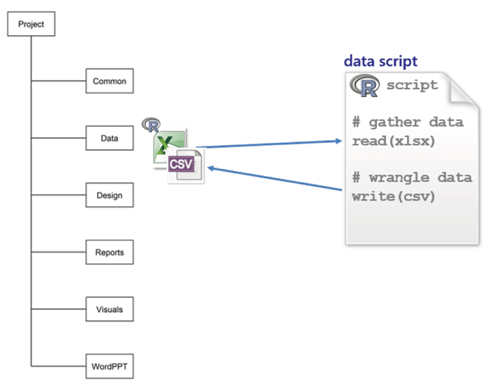
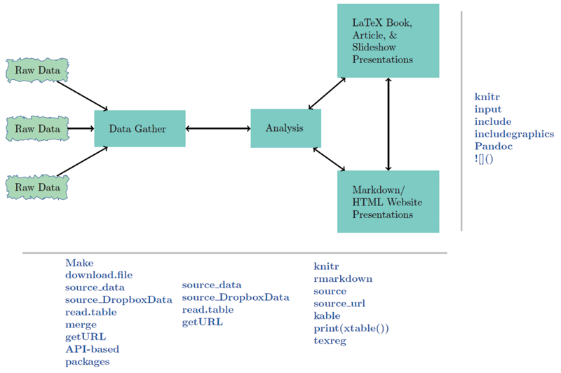
Gandrud identifies three main categories of work in computational research—data, analysis, and presentation. He recommends creating a project main directory with a sub-directory for each of the three categories. How the categories interconnect and the family of scripting commands used for each connection are illustrated in the figure, borrowed from Gandrud’s repository for the book’s second edition.
Gandrud describes how to use knitr and RStudio to perform commonly encountered tasks; for example, how to reproducibly obtain and manipulate data or how to get started with R Markdown (Rmd files) or LaTeX (Rnw files) for reproducible reporting. Gandrud covers task work in each area (data, analysis, and presentation). The book is written with a level of detail suitable for beginners in reproducible research.
<img src="http://chance.amstat.org/files/2015/11/bookfig2asmall.png" alt="Interconnections relating, data, analysis, and presentations. Christopher Gandrud. Reproducible Research with R and RStudio, 2/e. CRC Press, Taylor & Francis Group LLC, Boca Raton, FL, 2015.” width=”450″ height=”299″ class=”size-full wp-image-10193″ /> Interconnections relating, data, analysis, and presentations. Christopher Gandrud. Reproducible Research with R and RStudio, 2/e. CRC Press, Taylor & Francis Group LLC, Boca Raton, FL, 2015.One minor complaint. The enthusiasm with which Gandrud introduces make made me eager to give it a try, but I never quite figured it out. The barrier to understanding is partly my unfamiliarity with the make environment and partly that the topic is developed at a somewhat higher level than other topics in the book. This might be a case of unstated assumptions obvious to the author that are not obvious to the reader—always a hazard when the expert writes for the novice.
Nevertheless, this is a minor quibble. Gandrud’s work has had a significant and lasting effect on how I think about how my work flows. I highly recommend the book and I look forward to adding the second edition to my library.
Implementing Reproducible Research
Victoria Stodden, Friedrich Leisch, and Roger D. Peng
Hardback: 448 Pages
Year: 2014
Publisher: Chapman and Hall/CRC
ISBN: 9781466561595
In my opinion, everyone using R for reproducible research will want to read Xie and Gandrud cover-to-cover and more than once. In contrast, in the collection, edited by Stodden, Leisch, and Peng, some chapters are more engaging than others. All are well-written (and edited) but, like articles in conference proceedings, different chapters will appeal to different readers.
Nevertheless, because the book provides a broad view of the entire reproducible research landscape (circa 2014), every practitioner should find practical suggestions to apply in their own work, as well as thought-provoking propositions on the future of the field.
The book is divided into three major parts. Part 1, “Tools,” covers computational tools knitr, VisTrails, Sumatra, and others. Part 2, “Practices and guidelines,” covers open-source practice, good programming practice, open science, and cloud computing. Part 3, “Platforms,” covers software and platforms, including open-source software packages, the RunMyCode platform, and open-access journals.
While any published discussion of software becomes dated fairly quickly, the problems addressed by reproducible research persist, making the problem descriptions and solution methods by these authors of longer-lasting interest to readers. Parts of the book that spoke to me personally and influenced my work are chapters on knitr (Ch. 1), managing reproducibility for large-scale projects (Ch. 8), and intellectual property (Ch. 12).
Influences
Most readers will find some aspect of reproducible research to adopt to improve their work flow. Two ideas have most influenced my work: explicitly tying scripts together for reproducibility, and planning file management from the beginning of a project.
I have encountered a number of schemes for directory and file organization. Jenny Bryan, for example, has posted some good advice from her talk at the Reproducible Science Workshop. Or consider Peter Baker’s dryworkflow package for creating a complete project directory skeleton.
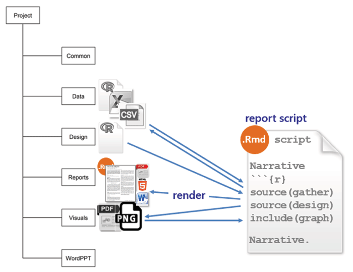
In my current work flow, I’ve modified Gandrud’s directory structure, expanding his three basic categories—data, analysis, and presentation—to the directory structure pictured.
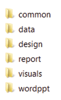
The main project directory contains these subdirectories. The design of a directory structure is highly personalized, but everyone agrees that planning the structure at the beginning of a project is necessary for reproducibility.
common is for document elements re-used from project to project, e.g., business logo, LaTeX preambles, bibliography files, reference styles documents for rendering R Markdown to MSWord, etc.
data is for data spreadsheets received from collaborators, original data sets from any source, and R scripts to gather, manipulate, and save tidy data, usually in CSV format. My scripts are self-contained so I can run them independently of any other work in the project.
Every script explicitly documents the links among files. For example, suppose I’m studying undergraduate graduation rates. I would write a script named gather-grad-rate-data.R to read and tidy the original data and write the resulting data frame to file.
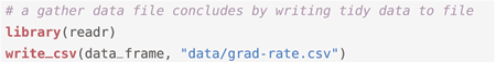
Because the project-level directory is the working directory, the filename includes the path to the data sub-directory.
Some data scientists recommend a separate directory for raw data to keep it in pristine condition. Others also recommend a separate directory for scripts that tidy the data. Everyone agrees, however, that you should pick a scheme—any scheme—and use it.
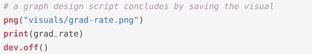
design is for scripts that read the prepared CSV data files, create graphs and tables, and write them to the visuals directory. These R scripts are also self-contained, so I can execute them independently while I’m designing and revising a graph. I prefer to call this directory “design” because my primary work is in creating graphs; others prefer “analysis.”

To illustrate, a design file grad-rate.R would begin by reading the CSV data file prepared earlier,

and would conclude with a graphics device statement such as:
reports is for Rnw or Rmd markup scripts that produce a reproducible report. For those of us not using a make file, this is the master script that invokes all the scripts required to render a report in the desired format, e.g., PDF, HTML, or MSWord.
If I’m the sole author, I use Rnw markup because I’m comfortable using LaTex and I enjoy the fine control it provides for document design. Also, some publishers provide LaTex style files, simplifying the task of conforming to their formatting requirements. I use Rmd markup when I have collaborators who use MSWord exclusively or when I’m writing something I plan to post to github.
In either case, the report script executes each independent data script and design script by name and includes the resulting tables and graphs in the report with accompanying narratives. I should note that, in this work flow, every script is executed every time I update a report. While not a problem for smaller data sets, this approach is computationally expensive for larger data sets. Gandrud (and others) recommend using make to save computational expense.
My report file usually includes the following option so that figures rendered by knitr are saved to the visuals directory:

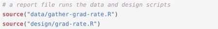
The report file executes the gather data script and the design script using the source() function:
If I’m reporting in Rnw format, my document preamble will set the path for visuals using:
![]()
and I can insert a graph in the report with:
![]()
If I’m reporting in Rmd format, I insert a graph with:
![]()
or use HTML syntax for greater control, where height and width are in pixels and the relative path to the visual file is explicit.
![]()
wordppt I regularly work with colleagues who do not work reproducibly—who regularly do analysis in Excel, reporting in Word, and presenting in PowerPoint. I save the materials they send me in this directory. If any of their work affects my reproducible work, I make the necessary updates and revisions to my scripts, re-run the main report, and send it to my collaborators.
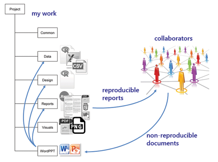
If I am in charge of the final report, it will be fully reproducible. If another member of the team is in charge of the final report and is not using reproducible practices, they will copy and paste elements from my work to import it to the final report. This introduces some non-reproducible steps into the work flow.
Hoefling and Rossinni, in Stodden, Leisch, & Peng, Chapter 8, have some perceptive insights on the problems of collaborating on large-scale reproducible projects. Some of the future improvements they wanted have been addressed since the book was published; e.g., if using RMarkdown to render a report to MSWord, we now have support for tables and MSWord style assignments for headers, footers, section headings, etc. Tables are now supported using the kable() function in knitr or pandoc arguments in RMarkdown.
Final Thoughts
Applying two basic principles for reproducible research—explicitly linking computing, results, and narrative, and organizing for reproducibility from the beginning of a project—has improved the productivity of my computational work and my contributions to collaborative research.
In retrospect, it seems astonishing that work flows like I’ve described here have only recently begun to be taught to students of science, engineering, and mathematics. As Millman and Perez put it (Stodden, Leisch, and Peng, Chapter 6):
Yet, for all its importance, computing receives perfunctory attention in the training of new scientists and in the conduct of everyday research. It is treated as an inconsequential task that students and researchers learn “on the go” with little consideration for ensuring computational results are trustworthy, comprehensible, and ultimately a secure foundation for reproducible outcomes. Software and data are stored with poor organization, little documentation, and few tests. A haphazard patchwork of software tools is used with limited attention paid to capturing the complex workflows that emerge. The evolution of code is not tracked over time, making it difficult to understand what iteration of the code was used to obtain any specific result. Finally, many of the software packages used by scientists in research are proprietary and closed source, preventing complete understanding and control of the final scientific result.
Anyone working to make their research reproducible will find abundant advice, practical suggestions, how-to examples, and ideas and issues to ponder in all three books. I have read and re-read them a number of times, and I look forward to Xie’s and Gandrud’s second editions.
About the Author
Richard Layton is a graduate of California State University, Northridge (1991), and the University of Washington (1993, 1995). Since 2000, he has taught in the mechanical engineering department at the Rose-Hulman Institute of Technology in Terre Haute, Indiana. He is interested in data visualization, communication and ethics in engineering, and student teaming, and is a member of the CATME development team. Layton teaches a data visualization/introduction to R course for math, science, and engineering students. In recent research collaborations, he has focused on “creating more effective graphs,” to borrow from Naomi Robbins, and gives workshops on graph design.

Book Reviews is written by Christian Robert, an author of eight statistical volumes. If you are interested in submitting an article, contact Layton at xian@ceremade.dauphine.fr.


