Howard Wainer and Donald B. Rubin

The best-laid schemes o’ mice an’ men
Gang aft agley,
An’ lea’e us nought but grief an’ pain,
For promis’d joy!
– Robert Burns (1785)

Rubin’s model for causal inference helps us design experiments to measure the effects of possible causes. In a 2014 CHANCE column, this was illustrated with a hypothetical experiment on how to unravel a causal puzzle of happiness. Is it really this easy? The short answer is, unfortunately, no. But in the practical world, more complicated than the one evoked in the proposed happiness study, Rubin’s model is even more useful. In this article we shall go deeper into the dimly lit practical world, where participants in our causal experiment drop out for reasons outside of our control. We will show how statistical thinking in general, and Rubin’s Model in particular, can illuminate it. But let us go slowly, and so allow time for our eyes to acclimate to the darkness.

Controlled experimental studies, are typically referred to as the gold standard for which all investigators should strive, and observational studies as their polar opposite, are pejoratively described as “some data we found lying on the street.” In practice they are closer to one another than we are often willing to admit. The distinguished statistician Paul Holland, expanding on Robert Burns, observed that,

“All experimental studies are observational studies waiting to happen.”

This is an important and useful warning to all who are wise enough to heed it. Let us begin with a more careful description of both kinds of studies.

The key to an experimental study is control. In an experiment, those running it control:

1. The treatment condition
2. The alternative condition
3. Who gets the treatment
4. Who gets the alternative
5. The outcome (dependent) variables

In an observational study, the experimenter’s control is not as complete. Consider an experiment to measure the causal effect of smoking on life expectancy. Were we to do an experiment, the treatment might be a pack of cigarettes a day for one’s entire life. The alternative condition might be no smoking. Then we would randomly assign people to smoke or not smoke, and the dependent variable would be their age at death.

Obviously, such an experiment is theoretically possible, but not practically, for we cannot assign people to smoke or not at random.¹ This is the most typical shortcoming of even a well-designed observational study. Investigators could search out and recruit treatment participants who smoke a pack a day, and also control participants who are non-smokers. And they could balance the two groups on the basis of various observable characteristics (e.g., they could have the same sex/racial/ethnic/age mix in both groups). But when there is another variable that is related to length of life that is not measured there may be no balance on it. Randomization, of course, provides balance, on average, for all such “lurking missing variables.”

This example characterizes the shortcoming of most observational studies—the possibility of lack of balance between the alternative and treatment conditions that is achieved (on average) in an experiment through randomization. It also makes clear why an observational study needs to collect lots of ancillary information about each participant so that the kind of balancing required can be attempted. In a true experiment, with random assignment, such information is (in theory) not required. Here enters Paul Holland’s comment.

Suppose some participants drop out of the study. They might move away, stop showing up for annual visits, decide to quit smoking (for the treatment condition) or start (for the control), get hit by a truck, or expire for some other reason unrelated to smoking. At this point the randomization is knocked into a cocked hat and we must try to rescue the study using the tools of observational studies. Such a rescue is impossible if we have not had the foresight to record all of the crucial ancillary information, the covariates, that are the hallmark of a good observational study.

Missing variables due to our inability to randomize have misled us in the past. For a long time, the effect of obesity on life expectancy was underestimated because smokers tended to both die younger and be more slender than nonsmokers. Hence the negative effect of smoking on life expectancy was conflated with the advantage of avoiding obesity. Experiments in which we randomly assign people to be obese or not are not possible. Modern research on the effects of obesity excludes participants who have ever smoked.

“I used to be Snow White, but I drifted.”
– Mae West

It is obvious now, if it hadn’t been already, that even the most carefully planned experiments with human beings get contaminated when carried out in the real world. And yet our goals for these experiments do not change. The issue is clear: how can we estimate causal effects when unexpected events intrude on the data collection, causing some observations to be missing.

Let us begin with a fundamental fact that no amount of verbal or mathematical legerdemain can alter: The magic of statistics cannot put actual numbers where there are none.²

And so, when we run an experiment and some of the subjects drop out, taking with them the observations that were to be the grist for our inferential mill, what are we to do? There are many ways to answer this question, but all that are credible must include an increase in the uncertainty of our answer over what would have been had the observations not disappeared.

Coronary Bypass Surgery: An Illuminating Example

What can be done when, because of clogged arteries that have compromised its blood supply, the heart no longer operates effectively? For more than 50 years one solution to this problem has been coronary bypass surgery. In this procedure, another blood vessel (often from the leg) is harvested and sewn into the heart’s blood supply, bypassing the clogged one. This is not minor surgery, and it carries substantial risks, usually greater to a patient who is not in robust health. Before recommending this procedure widely, it is crucially important to assess for each type of patient how much it is likely to help. So let us construct an experiment that would measure the size of the causal effects that such surgery has on the health of the patients after the treatment:

1. Treatment—Bypass surgery in addition to medication, diet, and a program of exercise.
2. Control—Medication, diet, and a program of exercise, but no surgery.
3. Subjects—Chosen in both groups at random from a pool of individuals judged to have one or more clogged arteries that supply the heart.
4. Outcome Measure—Success of the intervention judged by a “Quality of Life” (QOL) score based on both medical and behavioral measures taken one year after the surgery.

After the experiment has been set up, we look carefully at the effectiveness of the randomization to assure ourselves that both groups match in terms of age, sex, socio-economic status, smoking, initial QOL, and everything else we can think of. It all checks out and the experiment begins.

As the experiment progresses, some of the patients die. Some die before the surgery, some during, some afterwards. For none of these patients is follow-up QOL measured. What are we to do?

One option might be to exclude all of the missing patients from the analysis and proceed as if they had never been in the experiment. This approach is too often followed in the analysis of survey data in which there might be just a 20% response rate, but the results are interpreted as if they represented everyone. This is almost surely a mistake, and the size of the bias introduced is generally proportional to the amount of missingness. We know of one survey done by a company of its employees that tried to assess “engagement with the company.” They reported that 86% of those responding were “engaged” or “highly engaged.” They also found that only 22% of those polled were engaged enough to respond!

A second option in our bypass experiment might be to impute a value for the missing information. For the non-respondents in the engagement survey one might impute a value of zero engagement, but that is likely too extreme.

It is tempting to follow this approach with the bypass surgery experiment and impute a zero QOL for everyone who is dead. But is this true? For many people, being alive, regardless of condition, is better than the alternative. Yet there are a fair number who would disagree and would score “being dead” higher than some other miserable living situation, and construct living wills to enshrine this belief.

Let us begin our discussion with an analysis of artificial (but plausible) data from such an experiment, which we summarize in Table 1.

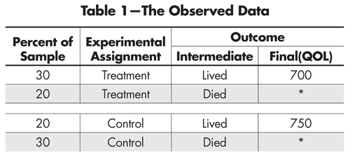
Table 1—The Observed Data

From this table we can deduce that 60% of those patients who received the treatment lived, whereas 40% of those who received the control survived. Thus, we would conclude that on the intermediate but still very important variable of survival, the treatment is superior to the control. But, among those who lived, the quality of life (QOL) of those who received the control condition was higher than among those who received the treatment (750 vs. 700).

We could easily have retrieved these two inferences from any one of dozens of statistical software packages, but this is a path that is fraught with danger. Remembering Picasso’s observation that for some things, “computers are worthless; they only give answers,” it seems wise to think before we jump to calculate and thence to conclude anything from these calculations.

We can believe the life vs. death conclusion because the two groups, treatment vs. control, were assigned at random. Thus we can credibly estimate that the size of the causal effect of the treatment relative to the control on survival is 60% vs. 40%. But the randomization is no longer in full effect when we consider the QOL, because the two groups being compared were not composed at random, for death has intervened in a decidedly non-random fashion. What are we to do?

Rubin’s Model provides clarity. One of the key pieces of Rubin’s Model is the idea of a potential outcome. That is, each subject of the experiment, before the experiment begins, has a potential outcome under the treatment and another under the control. The difference between these two outcomes is defined as the causal effect of the treatment, but we only get to observe one of those outcomes. This is why we can only speak of a summary causal effect, for example, averaged over each of the two experimental groups. And this is most credible with random assignment of subjects to treatment.

The bypass experiment has one outcome measure that we planned, the Quality of Life score (QOL), and a second—an intermediate outcome, life or death—which was unplanned. Thus for each participant we observe whether he or she lived. What this means is that the data fall into four conceptual categories, those who would:

1. Live with treatment and live with control
2. Live with treatment but die with control
3. Die with treatment but live with control
4. Die with treatment and die with control

Of course each of these four groups is itself randomly divided into two groups: those who actually got the treatment and those who got the control. So for category 1 we can observe their QOL score regardless of which experimental group they are in.

In category 2, we can only observe QOL for those who got the treatment, and similarly in category 3 we can only observe QOL for those who were in the control group. In category 4, which is probably made up of very fragile individuals, we cannot observe QOL for anyone.

This is summarized in Table 2, which makes it clear that if we simply ignore those who died we are comparing the QOL of those in cells (a) and (c) with that of those in (b) and (f). We are ignoring all subjects in (d), (e), (g) and (h). The four levels shown we shall call the “Survival Strata.”

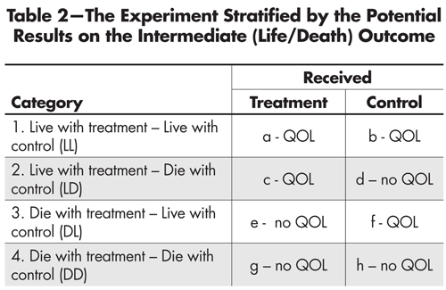
Table 2—The Experiment Stratified by the Potential Results on the Intermediate (Life/Death) Outcome

At this point three things are clear:

1. The use of Rubin’s idea of potential outcomes has helped us to think rigorously about the character of the interpretation of the experiment’s results.
2. It is only from the subjects in category 1 that we can get an unambiguous estimate of the average causal effect of the treatment on QOL, for it is only in this principal stratum that the QOL data in each of the two treatment conditions are generated from a random sample from those in that stratum.
3. So far we haven’t a clue how to decide whether a person who lived and got the treatment was in category 1 or category 2, or whether someone who lived and got the control was in category 1 or category 3. And, unless we can make this classification decision (at least on average), our insight is not fully practical.

Let us bypass the difficulties posed by point (3) for a moment and consider a supernatural solution. Specifically, suppose a miracle occurred and some benevolent deity decided to ease our task and provide us with the outcome data we require. Those results are summarized in Table 3.

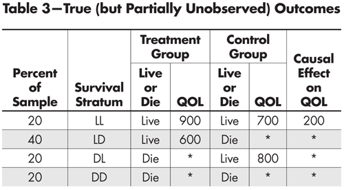
Table 3—True (but Partially Unobserved) Outcomes

It is unfortunate that the benevolent deity that provided the classifications in Table 3 didn’t also provide us with the QOL scores for all experiment participants, but that’s how miracles typically work,⁴ and we shouldn’t be ungrateful.

We can easily expand Table 3 to make explicit what is happening (see Table 4). For example, the first row can be broken into two rows, the first representing those participants who received the treatment and the second those who received the control. The rest of the entries are the same, except that some of them (in italics) are counterfactual given the experiment—what would have happened had they been placed in the other condition instead.

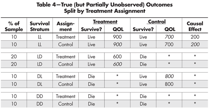
Table 4—True (but Partially Unobserved) Outcomes Split by Treatment Assignment

This expansion makes it clearer which strata provide us with a defined estimate of the causal effect of the treatment (LL) and which do not. It also shows us why the unbalanced inclusion of QOL outcomes from the LD and DL strata misled us about the causal advantage of the control condition on QOL.

“In the affairs of life, therefore, it is impossible for us to count on miracles or to take them into consideration at all…”
– Immanuel Kant (1724-1804)

The combination of Rubin’s Model (to clarify our thinking) and a minor miracle (to provide the information we needed to implement that clarity of thought) has guided us to the correct causal conclusions. Unfortunately, as Kant so clearly pointed out, although miracles might have occurred regularly in the distant past, they are pretty rare nowadays, and so we must look elsewhere for solutions to our contemporary problems.

Without the benefit of an occasional handy miracle, how are we to form the stratification that allowed us to estimate the causal effect of the treatment? Here enters Paul Holland’s aphorism again. If we were canny when we designed this experiment, we recognized the possibility that something might happen and so gathered extra information (covariates) that could help us if something happened to disturb the randomization.

How plausible is it to have available such ancillary information? Let us consider some hypothetical yet familiar kinds of conversations between a physician and a patient that might occur in the course of treatment.

1. “Fred, aside from your heart, you’re in great shape. While I don’t think you are in any immediate danger, the surgery will improve your life substantially.” (LL)
2. “Fred, you’re in trouble, and without the surgery we don’t hold out much hope. But you’re a good candidate for the surgery, and with it we think you’ll do very well.” (LD)
3. “Fred, for the specific reasons we’ve discussed, I don’t think you can survive surgery, but you’re in good enough shape so that with medication, diet, and rest we can prepare you so that sometime in the future, you will be strong enough for the surgery.” (DL)
4. (To Fred’s family) “Fred is in very poor shape, and there is nothing we can do that will help. We don’t think he can survive surgery, and without it, it is just a matter of time. I’m sorry.” (DD)

Obviously, each of these conversations involved a prediction, made by the physician, of what is likely to happen with and without the surgery. Such a prediction would be based on previous cases in which various measures of the patient’s health were used to estimate the likelihood of survival. The existence of such a system of predictors allows us, without the benefit of anything supernatural, to estimate each participant’s survival stratum.

Let us use a QOL measure of each participant’s health, taken as the experiment begins, as a simple pre-assignment predictor of survival stratum. We obtain this before there is an opportunity for any post-assignment dropouts.

Table 5 looks like Table 4, but has two critical differences. First, it includes the initial value of the QOL for each participant; and second, the determination of who was included in each of the survival stratum was based on how the value of the covariate relates to the intermediate (live/die) outcome, and not on the whim of some benevolent deity. More specifically, individual participants were grouped and then stratified by the value of their initial QOL score—no miracle required.

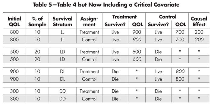
Table 5—Table 4 but Now Including a Critical Covariate

Those with very low QOL (300) were in remarkably poor condition and none of them survived regardless of whether they received the treatment. Those with high QOL (800) survived regardless of whether they received the treatment. Those with intermediate QOL scores (500) were not in very good shape and only survived if they had the treatment, whereas they perished if they did not. And last, those with very high QOL (900) pose something of a puzzle. If they were not treated, their QOL declined to 800, which is still not bad. But, if treated, they died. This is an unexpected outcome and requires follow-up interviews with their physicians and family to try to determine possible reasons for their deaths. Perhaps they felt so good after the treatment that they engaged in some too-strenuous activity that turned out to be fatally unwise.

Summary

“In the past, a theory could get by on its beauty; in the modern world, a successful theory has to work for a living.”

1. Before assignment in an experiment, each subject has two potential outcomes—one under the treatment and the other under the control.
2. The causal effect of the treatment (relative to the control) is defined as the difference between these two potential outcomes.
3. The fly in the ointment is that we only get to observe one of these.
4. We get around this by estimating the average causal effect, and through random assignment, we make credible the assumption that what we observed among those in the control group is what we would have observed in the treatment group had they not gotten the treatment.
5. When someone dies before we can measure the dependent variable (QOL), we are out of luck. Thus the only people who can provide estimates of the causal effect are those who would have lived under the treatment and who would have lived under the control. No others could provide us with the information required.
6. So subjects who would survive under the treatment but not the control are no help; the same goes for those who would die in the treatment but not the control; and, of course those who would die under both conditions add nothing.
7. So we can get an estimate of the causal effect of the treatment only from those who would survive under both conditions.
8. But we don’t get to observe whether they will survive under both—only under the condition to which they were assigned.
9. To determine if they would have survived under the counterfactual condition, we need to predict that outcome using additional (covariate) information.
10. If such information doesn’t exist, or if it isn’t good enough to make a sufficiently accurate prediction, we are stuck. And no amount of yelling and screaming will change that.

Conclusion

In this essay we have taken a step into the real world where even randomized experiments can be tricky to analyze correctly. Although we illustrated this with death as the very dramatic reason for non-response, the case we sketched occurs frequently in less dire circumstances. For example, a parallel situation occurs in randomized medical trials comparing a new drug with a placebo, where if the patient deteriorates rapidly, rescue therapy (a standard, already approved drug) is used. As we demonstrated here, and in that context as well, one should compare the new drug with the placebo on the subset of patients who wouldn’t need rescue whether assigned the treatment or a placebo.

These are but a tiny sampling of the many situations in which the clear thinking afforded by Rubin’s Model—with its emphasis on potential outcomes—can help us avoid being led astray. We also have emphasized the crucial importance of covariate information, which provided the pathway to forming the stratification that revealed the true value of the causal effect. For purposes of cogent and concise description, we have used a remarkably good covariate (initial QOL) that made the stratification of individuals unambiguous. Such covariates are welcome but rare. When such collateral information is not quite so good, we will need to use additional techniques, whose complexity doesn’t lend themselves easily to the goals of this discussion.

What we have learned in this exercise is that:

1. The naïve estimate of the causal effect of the treatment on QOL, derived in Table 1, was wrong.
2. The only way to get an unambiguous estimate of the causal effect was by classifying the study participants by their potential outcomes, for it is only in the survival stratum occupied by participants who would have lived under either treatment or control that such an unambiguous estimate can be obtained.
3. Determining the survival stratum of each participant can only be done with ancillary information (here their pre-study QOL). The weaker the connection between survival stratum and this ancillary information, the greater the uncertainty in the estimate of the size of the causal effect.
4. This was a simplified and contrived example, but the deep ideas contained are correct, and so nothing that was said needs to be relearned by those who choose to go further.

Further Reading

Kant, I. 1960. Religion Within the Limits of Reason Alone, 2nd ed. Translated by T. M. Green and H. H. Hudon. New York: Harper Torchbook.

Kitahara C. M., et al. July 8, 2014. Association between class III obesity (BMI of 40–59 kg/m) and mortality: a pooled analysis of 20 prospective studies. PLOS Medicine. DOI: 10.1371/journal.pmed.1001673.

Rubin, D. B. 2006. Causal inference through potential outcomes and principal stratification: Application to studies with “Censoring” due to death. Statistical Science 21(3): 299-309.

Wainer, H. 2014. Happiness and Causal Inference. CHANCE 27(4): 61-64.

¹This experiment has been attempted with animals, where random assignment is practical, but it has never shown any causal effect. This presumably is because easily available experimental animals (e.g. dogs or rats) do not live long enough for the carcinogenic effects of smoking to be manifested, and animals with long-enough lives (e.g., tortoises) cannot be induced to smoke.
²We suspect that this has been stated many times by many seers, but my source of this version was from a prince of statistical aphorisms, Paul Holland.
³Man plans and God laughs. In the original Yiddish,
⁴History is rife with partial miracles. Why mess around with seven plagues, when God could just as easily have transported the Children of Israel directly to the Land of Milk and Honey? And while we’re at it, why shepherd them to the one area in the Middle East that had no oil? Would it have hurt to whisk them instead directly to Maui?

About the Authors

Howard Wainer is distinguished research scientist at the National Board of Medical Examiners. He has won numerous awards and is a Fellow of the American Statistical Association and American Educational Research Association. His interests include the use of graphical methods for data analysis and communication, robust statistical methodology, and the development and application of generalizations of item-response theory. He has published 20 books so far; his latest is Medical Illuminations: Using Evidence, Visualization & Statistical Thinking to Improve Healthcare (Oxford University Press, 2014).

Donald Bruce Rubin is the John L. Loeb Professor of Statistics at Harvard University. He was hired by Harvard in 1984, and served as chair of the department for thirteen years. He is possibly most well known for the Rubin Causal Model, a set of methods designed for causal inference with experimental or observational data, and for his methods for dealing with missing data.

Visual Revelations covers many topics, but generally focuses on two principal themes: graphical display and history. Howard Wainer, column editor, encourages using this column as an outlet for popular statistical discourse. If you have questions or comments about the column, please contact Wainer at hwainer@nbme.org.

Back to Top