
Streakiness in Home Run Hitting

Sports fans are fascinated with patterns of hot and cold behavior among athletes and teams. One of the greatest hitting accomplishments in baseball is Joe DiMaggio’s “Great Streak” of getting a hit in 56 consecutive games in the 1941 season. The Oakland Athletics’ winning streak of 20 consecutive games during the 2002 baseball season was partly the inspiration for the book and movie Moneyball. Indeed, streaky patterns of performance have been featured in a number of CHANCE articles. In baseball, some of the best-known hitters are the ones who hit a large number of home runs during a season. Albert Pujols won the MVP (most valuable player) award in the 2009 season partly due to hitting 47 home runs. Likewise, Mo Vaughn’s 40 home runs contributed to his fourth place in the voting for the MVP crown in the 1998 season. But the 2009 Pujols and the 1998 Vaughn had different patterns of home run hitting during these two seasons.
In 2009, Albert Pujols had 10 occurrences when he hit home runs in consecutive at-bats (opportunities), and there were periods of 62 at-bats and 79 at-bats during the season in which he failed to hit a single home run. Pujols clearly demonstrated a streaky pattern of home run hitting in the 2009 season. In contrast, Vaughn in 1998 only had a single occurrence of hitting back-to-back home runs, and his longest drought of home run hitting was only 43 at-bats. The 1998 Vaughn appeared to be more consistent or less streaky than the 2009 Pujols in home run hitting.
This brief anecdote raises the following questions about streaky patterns:
- How does one measure streaky behavior?”
- Can one define what it means to be a consistent home run hitter during a season?”
- What does it mean to be “truly” streaky?
- What type of streaky patterns in home run hitting does one expect by “chance”?
- Is there a way of measuring the degree of true streakiness in home run hitting?
- Are there players in Major League Baseball history who tend to be unusually consistent or streaky in their home run hitting?
Looking at Spacings
Pujols had 568 official at-bats during the 2009 season. (By considering official at-bats, we are discarding plate appearances such as walks and hit-by-pitches in which the batter does not have an opportunity to hit a home run.) Suppose we record the numbers of the at-bats where Pujols hit his home runs and consider the spacings, the number of at-bats between consecutive home runs. Here are the spacings for Pujols in the 2009 season:
4,14,0,4,28,1,8,13,3,10,
0,14,1,28,19,1,15,4,21,2,3,
0,5,9,3,0,18,0,7,0,7,20,
14,0,62,0,21,2,14,1914,8,
13,0,11, 2, 0, 79
From these spacings, we see Pujols had four “homerless” at-bats until his first home run, he went 14 at-bats until his next home run, he hit two consecutive home runs, he went four at-bats until his next home run, and so on. Pujols streaky pattern of hitting home runs is indicated by the 10 “0” spacings (corresponding to the 10 back-to-back home runs) and the large spacing values of 62 and 79.
Figure 1 shows parallel histograms of the home run spacings of the 2009 Pujols and 1998 Vaughn. We see the large number of 0 spacings and the two large spacings for Pujols. In contrast, the spacings for Vaughn are concentrated between the values 5 and 30, and he had few large spacings and few spacings near zero.
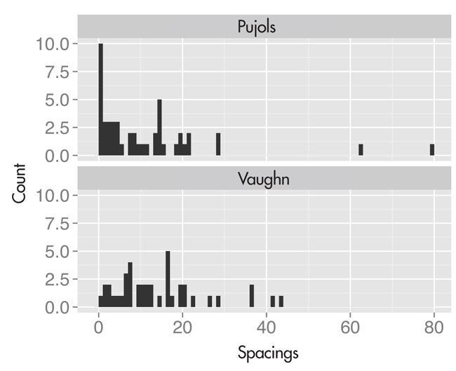
Figure 1. Histograms of spacings between home runs for the 2009 Albert Pujols and the 1998 Mo Vaughn. Pujols’s spacings indicate more streakiness by the large number of zero spacings and several large spacings.
Consistent and Streaky Models for Home Run Hitting
One can better understand the distribution of spacings by introducing several probability models for home run hitting. First let’s define the ultimate consistent home run hitter. This hitter has a fixed unknown probability, call it p, of hitting a home run on every at-bat, and the outcomes on different at-bats are independent. The pattern of home run hitting of this consistent hitter is analogous to the pattern of repeated flips of a biased coin where the chance of obtaining heads on a single flip is p. For this “consistent” hitter, statisticians are familiar with the distribution of spacings—the individual spacings are independent from a geometric distribution with probability p.
A geometric distribution with a constant hitting probability describes the pattern of spacings when the hitter is a true consistent hitter. What if a hitter is truly streaky? One way of understanding streakiness is to relax the assumption that the hitter has a constant home run probability. One possible “streaky alternative” is that the hitter has periods in which he is cold and hits a home run with probability pC and other periods where he is hot and is successful with probability pH where pC < pH. Another possible streaky alternative considered here is that the batter’s home run probabilities for the observed spacings change across the season and the collective probabilities have a density with an unknown mean M and parameter K. One reflects the lack of knowledge about the mean M by means of a flat or uninformative probability density. This parameter K controls the spread or variability of the home run probabilities—as one decreases K, the home run probabilities become more spread out. Figure 2 graphically shows these distributions of home run probabilities under the consistent model and two streaky models for two choices of the parameter K. For this particular player, he is consistent if he hits home runs with a constant probability of 0.083. This player is moderately streaky if his home run probabilities, with K = 148, have a small spread about 0.083, and is very streaky if his success probabilities, with K = 50, have a large spread about 0.083.
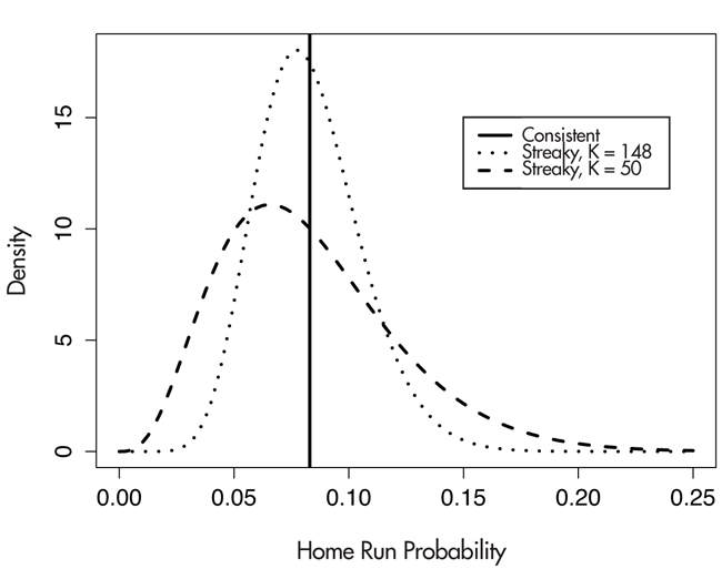
Figure 2. Distributions of home run probabilities under consistent and two streaky models. If Albert Pujols is truly consistent, then his probability of hitting a home run on every at-bat is a constant value (here assumed to be 0.083). In contrast, under the “K = 148” streaky model, the home run probabilities during the season vary around the value 0.083, and the “K = 50” model indicates even more variability about the value 0.083.
A Statistical Test of Consistent and Streaky Models
Now that we have two potential probability models, a consistent model and a streaky model, for describing the pattern of spacings between home run events, a Bayes factor provides a general way of assessing the relative support of the data for the two models. (A brief introduction to a Bayes factor is given in the sidebar.) The Bayes factor in support of the streaky model over the consistent model is given by the ratio
BFSC = f(data | MS) / f(data | MC),
where f(data | MS) is the predictive probability of the spacings values under the streaky model and f(data | MS) is the probability of the spacings under the consistent model. A value of BFSC > 1 indicates support for the streaky model and, likewise, BFSC < 1 indicates support for the consistent hitting model.
To compute a Bayes factor in practice, one needs to specify the parameter K that indicates the variability of the home run probabilities throughout a season if the player is truly streaky. In this application, we specify the value K = 148 reflecting the belief that Pujols’ home run probability (if he were truly streaky) ranges between the values 0.038 and 0.128 during the season. Using this value of K, we find the Bayes factor in support of the streaky model over the consistent model is BFSC = 3.6 for the 2009 Pujols, and the same measure for the 1998 Vaughn is BFSC = 0.39. These test statistics confirm the patterns we saw in the spacings. There is evidence Pujols was truly streaky in his home run hitting in this particular season. Likewise, there is evidence from the Bayes factor calculation that Vaughn was truly consistent in hitting home runs (relative to the streaky model) in the 1998 season.
Are These Streaky Patterns Predictable by Chance?
Although the Bayes factor is a useful measure of streaky behavior, it is unclear that statisticians should care about this exploration. After all, it is well known that even coin tossing can occasionally display streaky patterns, and so it is unclear whether our investigation has found more streakiness than one would anticipate if we were flipping a group of biased coins.
To address this concern, we ran a simulation. In the 2012 baseball season, we found 17 players (among all the players with at least 200 at-bats) who displayed “significant” streaky home run hitting, where significant was defined to be a Bayes factor exceeding 1.65. (The value 1.65 was chosen in an arbitrary manner to separate out a small number of players with streaky hitting patterns.) Suppose all the hitters this season had constant home run hitting probabilities—would it be surprising to find 17 streaky hitters?
We ran a simulation in which individual at-bat results were simulated for all the batters with at least 200 at-bats, assuming each hitter had a constant home run probability. The constant home run probabilities were estimated by shrinking or adjusting the observed home run rates toward a common value. For each simulation, the number of hitters displaying streakiness was recorded, and by repeating the simulation for many seasons, one can obtain the distribution of the number of streaky hitters under the consistent hitting model. If the actual number of streaky home run hitters in the 2012 season, 17, is in the right tail of this distribution, this indicates there was indeed more streakiness in this season’s data than one would predict by chance.
This simulation process was repeated for each of the baseball seasons 1960 to 2012. Figure 3 displays the mean plus and minus the standard deviation of the number of streaky hitters predicted under the biased coin model, and the actual number of streaky hitters for all seasons are overlaid on the display with solid dots. There are several interesting observations we can make when viewing this figure:
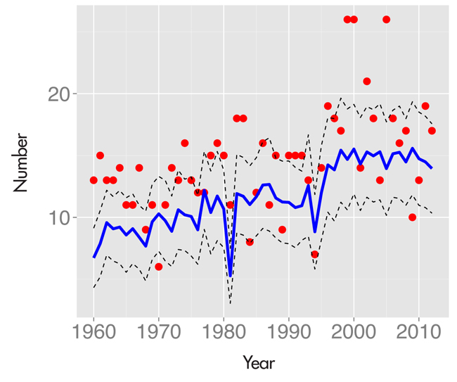
Figure 3. The blue line represents the mean number of predicted streaky hitters (using our Bayes factor measure) for each baseball season from 1960 through 2012 if each player had a constant season home run probability. The dotted lines present error bars (the mean plus and minus the standard deviation) for these predictions. The dots represent the actual number of streaky home run hitters for these seasons. Since the dots generally fall in the right tail of the predictive distribution, this indicates we are observing more streakiness than one would predict by chance.
- The number of streaky hitters under the consistent model has generally increased from 1960 to 2012. This pattern is likely due to the increase (due to expansion) of the number of players with at least 200 at-bats.
- In the simulation, there was a substantial drop in the number of streaky hitters in 1981 and 1994. This is likely due to a general drop in the rate of home run hitting during these seasons.
- The largest numbers of observed streaky hitters occur near the 2000 season, which corresponds with the period when there was alleged widespread use of steroids in baseball.
- Since most of the observed numbers of streaky hitters fall above the upper curve, we conclude there is indeed more streaky behavior in the actual home run hitting data than one would predict if the hitters were acting like a collection of biased coins.
This is an interesting conclusion—there is more observed streakiness in baseball home run hitting than one would predict by chance.
A Historical View of Streakiness
We have a useful tool for detecting streakiness on the basis of a collection of spacings. Also, we have evidence the streaky behavior observed in the 1960 to 2012 seasons is meaningful in that it exceeds the streaky behavior from a collection of biased coins. Continuing our exploration, we use our Bayes factor test to explore the streaky patterns of home run hitting for the 14,077 player seasons between 1960 and 2012. We focus on unusually streaky and unusually consistent patterns of home run hitting. In addition, we search for hitters who appear to be streaky or consistent for large portions of their careers.
Two Interesting Patterns of Home Run Hitting
Suppose we focus our streaky search to the player seasons with at least 40 home runs—there were 235 of these seasons between 1960 and 2012. Of these seasons, the 2002 Shawn Green had one of the most remarkable streaky home run hitting seasons—the Bayes factor in support of streakiness was 5.05.
Here are Green’s home run spacings during this season (the at-bat locations of his home runs are displayed in the top panel of Figure 4):

Figure 4. Plots of the location of at-bats of the home runs hit during Shawn Green’s streaky 2002 season and Hank Aaron’s consistent 1963 season
23,13,27,91,1,5,0,0,1,0,4,0,9, 30,7,7,3,0,0,0,8,10,5,6,2,
16,17,68,12,2,13,3,1,2,12,
10,14,3,26,9,16,6,58
In this particular season, Green hit seven home runs in one sequence of 12 at-bats and had a second non-overlapping hot period of five home runs in 12 at-bats. In contrast, 1963 Hank Aaron had the most consistent home run hitting season; the Bayes factor in support of the streaky model was 0.36, so this statistic favored the consistent model. (See the bottom panel of Figure 4.) Aaron’s home run spacings for the 1963 season have an interesting pattern:
11,25,4,9,3,11,9,9,3,11,
11,21,4,13,19,2,38,19,11,
24,14,3,18,9,33,6,
27,5,16,35,30,11,1,19,14,4,14,
1,1,14,32,9,3
In sharp contrast with Green, Aaron’s longest homerless streak was only 38 at-bats.
Career Streakiness: Carl Yastrzemski and Hank Aaron
We see that particular players had unusual patterns of home run hitting during specific seasons. But if a player is called a “streaky hitter,” then one would expect him to display a streaky pattern of home run hitting over multiple seasons. We did a search across the seasons 1960 through 2012 to find players who displayed a number of streaky home run hitting seasons (where “streaky” is defined as a Bayes factor exceeding 1.65).
One interesting career streaky hitter was Carl Yastrzemski, the Boston slugger who played between 1961 and 1983. For each season of Yastrzemski’s career, the Bayes factor in support of streakiness was computed, and the top panel of Figure 5 plots the Bayes factor (on a log scale) against season. Yastrzemski displayed seven seasons of streaky hitting, and four of the seven streaky seasons occurred during the middle of his career between 1972 and 1976.

Figure 5. The log Bayes factor in support of streakiness for the home run data of Carl Yastrzemski (top) and Hank Aaron (bottom) for all seasons of their careers. “Yaz” displayed a pattern of streaky hitting during the middle of his career; in contrast, “Hammerin’ Hank” had a consistent pattern of hitting home runs during his career.
In contrast, Aaron displayed a different pattern of home run hitting. Looking at the log Bayes factor in support of streakiness (see the bottom panel of Figure 5), we see Aaron had a consistent pattern of home run spacings for all seasons in his career. It is well known that Aaron had consistent home run totals for the seasons in his career. For example, in the period between 1957 to 1973, Aaron had 13 seasons in which he hit between 34 and 47 home runs. But this work also tells us that Aaron’s pattern of home run hitting within each season was consistent.
Concluding Comments
In sports, one observes many streaky performances among players, and the objective of this article is to see what these streaky performances tell us about the “streaky abilities” of players. We focus on the spacings between consecutive home runs and measure consistent and streaky abilities by means of distributions placed on the underlying home run probabilities. A Bayes test statistic was used to measure the support for true streakiness from a pattern of spacings, and this measure was helpful in finding players who had unusually streaky and consistent home run hitting seasons.
Of course, when one looks at many hitters over many seasons, one will find a number of streaky home run hitting seasons. But one interesting finding is the number of streaky performances exceeds what one would expect by chance; in other words, the number of observed streaky hitters exceeds what one would predict if all players had constant home run hitting probabilities. However, despite the media’s classification of hitters as “streaky,” it appears difficult to find specific hitters who are streaky for many seasons during their careers.
One can predict that streakiness of athletes will continue to be a popular topic for investigation, and I imagine there will be many future CHANCE articles on the hot hand. One challenge of this research is to get better measurements on the size of a player’s streaky ability and find athletes who have genuine streaky tendencies throughout their careers.
Editor’s Note: This article is based on the talk “Assessing Streakiness in Home Run Hitting,” presented by Jim Albert at the 2013 New England Symposium on Statistics in Sports. View the talk on YouTube.
Further Reading
Albert, Jim. 2004. Streakiness in team performance. CHANCE 17(4):37–43.
Albert, Jim. 2013. Looking at spacings to assess streakiness. Journal of Quantitative Analysis 9(2):151–163.
Berry, Scott. 1991. The summer of ’41: A probabilistic analysis of DiMaggio’s streak and Williams’ average of .406. CHANCE 4(4):8–11.
Gould, Stephen Jay. 1989. The streak of streaks. CHANCE, 2(2):10–16.
Stern, Hal S. 1997. Judging who’s hot or who’s not. CHANCE 10(2):40–43.
Tversky, Amos, and Thomas Gilovich. 1989. The hot hand: Statistical reality or cognitive illusion? CHANCE 2(4):31–34.
About the Author
Jim Albert is professor of statistics at Bowling Green State University. His interests include Bayesian modeling, statistics education, and the application of statistical thinking in sports. He is concluding his term as editor of the Journal of Quantitative Analysis of Sports. His most recent book is Analyzing Baseball with R. He is fortunate to have witnessed two World Series championships for his Phillies, 1980 and 2008.


