
Can Tax Deadlines Cause Fatal Mistakes?

Taxation has been a contentious issue in the United States for centuries (Figure 1). In particular, personal income tax deadline day is an infamous stress for millions of Americans that now occurs each year in April. Many studies have explored how income tax payments might influence the longterm health of the United States economy; however, no study has tested how income tax deadlines might change the immediate health of individuals. We wondered whether the widespread stress throughout the community could increase the short-term risk on tax day of a fatal human error. Adverse stress is often blamed as a cause of human disease, yet such links are difficult to prove using an ordinary ethical experiment.
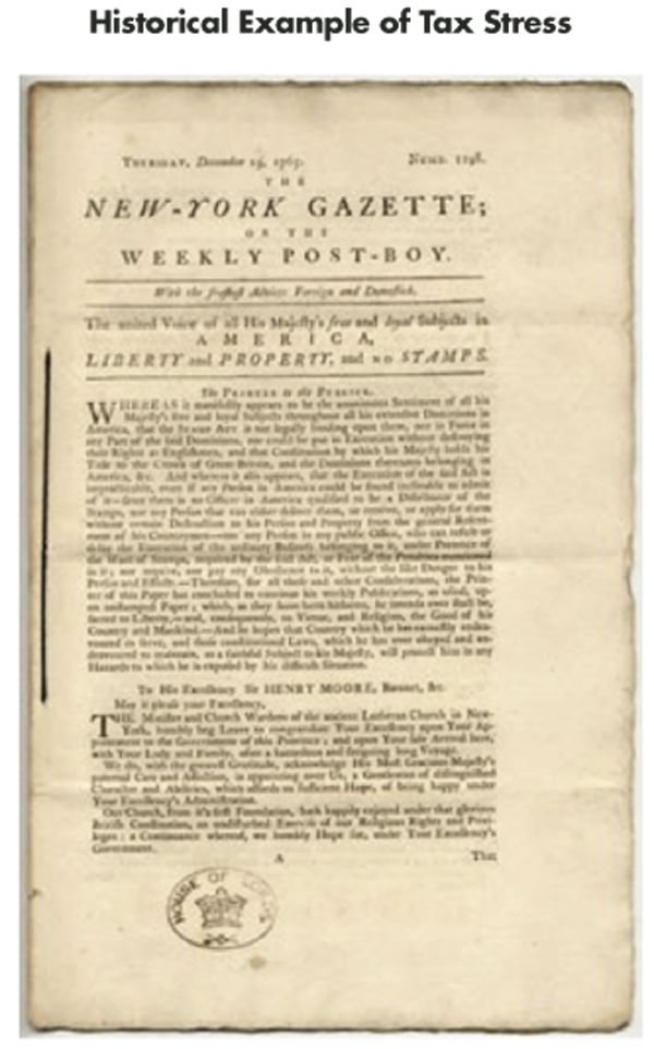
Figure 1. Photograph showing front page of The New York Gazette of Thursday, December 19, 1765. Article describes growing American colonial discontent toward increasing British parliamentary taxation. At the time, new taxes were initiated to defray costs of securing the empire and involved duties around stamping public documents (including legal papers, newspapers, and playing cards). An example of such stamping appears at lower left of the page. The discontent would contribute to the outbreak of the American Revolution in subsequent years.
The driving environment presents an intriguing domain for studying human error because the mistakes can be objective, compelling, and irreparable. Vehicle traffic also offers a huge sample size based on about 200 million licensed drivers traveling 3 trillion miles in the United States annually (equal to the distance traveled by a beam of light in six months). Vehicle traffic, furthermore, is amenable to scientific scrutiny since major mistakes are a matter of public record, do not rely on self-report, and reflect dangers that are impossible to mimic in a laboratory. The driving environment also holds widespread interest, since the average American spends a great deal of their entire lifetime confined to traveling in a vehicle.
Human error in the driving environment leads to about 40,000 road crashes each day in the United States. Even a small change in risk is important given these high baseline rates, wide population involvement, signficant counts of deaths, and additional numbers of individuals surviving with injuries or property loss. A 1% increase in relative risk during a single day in the United States, for example, leads to average economic losses of $6.3 million to society. Timely safety reminders can save lives, whereas shortfalls in prevention can cost them. The magnitude of mortality and morbidity attributable to road crashes is now especially high in the United States relative to other industrialized countries.
Analysis
We retrieved driving safety information for the United States from the National Highway Traffic Safety Administration. This information was accrued from the Fatality Analysis Reporting System website, a population-based database that includes all fatal crashes involving a motor vehicle on public roads throughout the United States (including the U.S. Virgin Islands). The database was public, freely available, and validated in past research on traffic fatalities. The database focuses only on fatal crashes and has important limitations due to a lack of data on driver education, medical history, distance traveled, and financial accounting.
Crash year, month, day, and location were recorded in all cases. Age, sex, and time were missing for some individuals (2.5%, 1.4%, 0.5%, respectively), and we coded such cases with modal values so that no person was excluded from subgroup analyses (reanalyzing after excluding such cases made no material difference). Alcohol level was missing in many cases (47%) and coded as “positive,” “negative,” or “unknown.” Position was defined as “driver,” “passenger,” or “pedestrian,” with miscellaneous cases coded as the first category. Early outcome was defined by initial status as “alive” or “dead” with missing data assumed as alive at the scene (since a fatal crash does not always kill all those involved).
We identified tax deadline data from the Internal Revenue Service. Dates spanned the full study interval with no years missing. For each tax day, we identified controls as the day one week before and one week after; for example, tax day of April 15, 2009, was matched to control days of April 8, 2009, and April 22, 2009. This approach controlled for year, month, and weekday, as well as reduced confounding from differences in roadway layout, vehicle technology, driver training, gasoline prices, prevailing laws, human genetics, health care access, population demographics, and many other influences on road trauma.
Our primary analysis used a binomial approximation to evaluate the total number of people in fatal crashes on tax days compared to control days. Doing so essentially examined departures from a ratio of 1:2 (each tax day has two controls), since the crash database was large and no days were missing (tax day has never been cancelled). The main advantage of this approach was that it is simple to program, easy to repeat, and readily generated odds ratio measures of relative risk along with 95% confidence intervals. The binomial approximation is sufficiently simple that it can be checked with a hand-held calculator (Figure 2).

Figure 2. Upper panel shows a 2×2 table correlating exposure with outcome (using counts of persons with corresponding features). Estimated odds ratio (r) from formula r=ad/bc. Variability (v) from formula v=sqrt(1/a +1/b +1/c +1/d). Dispersion (w) from formula w=exponential(1.96 x v). Upper and lower bounds of 95% confidence interval of the odds ratio estimate given by inflating or deflating estimate by dispersion. Lower panel provides counts for a hypothetical community of about 1 million (M) drivers, about 10 million driver-days of observation for exposure, about twice as many driver-days of observation for control, and yet more crashes on exposure days than control days. In this case, r=4.00, v=0.12, w=1.27, and 95% confidence interval spans from 3.15 to 5.09. Recall that a binomial approximation is valid when comparing observed counts that are each sums of independent and identically distributed binary random variables. For calculations, we assume twice as many control days as tax days (d ≈ 2 x c) and a large population (1/c ≈ 0, 1/d ≈ 0).
A binomial test examines whether observed counts agree with random chance. Consider, for example, a single hypothetical year in which 200 persons were in fatal crashes on tax day and 100 persons were in fatal crashes on the two total control days (average 50 per day). These data would indicate a four-fold risk increase on tax day (200/50) equal to an odds ratio of 4.00 (95% confidence interval: 3.15 to 5.09). Notice how the matching connects the full day (not individual persons), the two control days provide power and balance (relative to a single control day), and tax day appears significantly risky (relative to a null odds ratio of 1.00).
In our study, we observed a total of 19,541 individuals involved in fatal crashes during the 30 tax days and 60 control days (Figure 3). The modal person was a young man driving in a rural location. The 30 tax days accounted for 6,783 individuals in fatal crashes, equivalent to 226 per day. The 60 control days accounted for 12,758 individuals in fatal crashes, equivalent to 213 per day. Comparison of tax days to control days using the binomial test yielded an odds ratio of 1.06 (95% confidence interval: 1.03 to 1.10; p<0.001) equal to an absolute increase of 404 individuals in fatal crashes on tax days over the study.

Figure 3. Upper panel for tax days and lower panel for control days. X-axis denotes grouping into five intervals of width 50 and spanning full range (minimum = 126, maximum = 348). Y-axis for count of days with corresponding number of persons (scale differs in panels since 1:2 ratio of tax days to control days). Distribution for tax days based on 6,783 individuals over 30 days (mean = 226.1 per day). Distribution for control days based on 12,758 individuals over 60 days (mean = 212.6 per day). Results show rightward shift in distribution where tax days more likely to have higher counts than control days.
We next examined a restricted analysis to account for the clustered nature of the data (individuals were nested in vehicles and vehicles nested in crashes). That is, the observations were not fully independent. We therefore confined our analysis to the 6,514 drivers who died in fatal crashes on the 30 tax days and 60 control days. The 30 tax days accounted for 2,252 drivers who died in crashes, equivalent to 75 per day. The 60 control days accounted for 4,262 drivers who died in crashes, equivalent to 71 per day. Comparison of tax days to control days yielded an odds ratio of 1.06 (95% confidence interval: 1.01 to 1.11).
We also applied an alternative statistical test to account for the serial nature of the data (individuals were accrued over successive years characterized by increasing vehicle technology, fuel prices, and other temporal trends). We therefore preserved the matching of each tax day with control days and then, each year, counted the observed number of individuals on tax day compared to the expected number of individuals on tax day (calculated as the mean of the two corresponding control days). The arithmetic difference between observed and expected counts could then be subjected to a paired t-test based on 30 separate observations.
We found that the total number of individuals in fatal crashes on tax day differed over the years. The safest tax day was April 15, 2009, with 153 total individuals in crashes. In contrast, the safest control day was April 8, 2009, with 126 total individuals in crashes. The observed and expected counts were calculated for each year and showed the highest increase for 2003, with 68 extra individuals on tax day. Evaluation of all years using the paired t-test yielded a mean increase of 13.5 extra individuals (95% confidence interval: 1.8 to 25.1), equal to an odds ratio of 1.06 (95% confidence interval: 1.01 to 1.11).
Subgroup analysis provided an additional method for testing the robustness of our results for persons with diverse characteristics. We found that the relative increase in risk was mostly apparent during the last 20 years and mostly related to adults under the age of 65 years (Figure 4). The increase in risk persisted in different regions, locations, hours, sexes, early outcomes, and alcohol levels. The increase in risk extended to passengers and pedestrians, although the 95% confidence intervals were broad. All subgroups overlapped the main analysis, and none showed a significant contrary result.
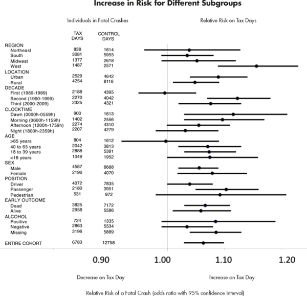
Figure 4. Forest plot of individuals in fatal road crashes over 30 years. X-axis shows relative increase in risk on tax days compared to control days expressed as odds ratio. Y-axis denotes subgroup (results for full cohort in final row). Column data are counts of individuals in crashes. Analytic results expressed with 95% confidence intervals setting control days as referent. Results show increased risk on tax day for full cohort, similar increase for 25 of 27 subgroups, and all confidence intervals overlapping main analysis. Recall that odds ratios are reliable estimates of relative risk when event rates are low from an individual driver’s perspective.
We further assessed robustness using tracer analyses. To do so, we identifed the day immediately before the tax deadline for comparisons to matched control days; for example, April 14, 2009, was matched to control days of April 7, 2009, and April 21, 2009. An analogous approach identified the day immediately after the tax deadline for comparisons to controls; for example, April 16, 2009, was matched to control days of April 9, 2009, and April 23, 2009. These analyses examined the specificity of the tax deadline and possible offsetting changes in surrounding days (that are often weekends or holidays).
We found that the day before the tax deadline averaged about 240 individuals per day, with no increase in risk compared to corresponding control days (odds ratio = 0.98, 95% confidence interval: 0.94 to 1.01). The day after the tax deadline averaged about 239 individuals per day, with no increase in risk compared to corresponding control days (odds ratio = 0.98, 95% confidence interval: 0.95 to 1.02). These analyses indicate the increased risk on tax days was distinct and not offset by surrounding days. The data also underscore how scheduling tax day on weekdays has safety advantages (since weekends have higher baseline risks).
Interpretation
Several reasons might explain why tax deadlines lead to increased road risks. One explanation is that stressful deadlines contribute to driver distraction and human error. Another might be more driving, yet we observed an increase rather than a decrease during recent decades when individuals can file electronically. A third explanation might relate to alcohol, although we found no accentuation during night hours, when alcohol consumption tends to be more common. Additional reasons might include sleep deprivation, decreased hazard monitoring, attentional failures, and less tolerance toward hassles.
Perhaps the largest limitation of our study is that we examined tax day to draw inferences over all days of the year. Tax deadlines are not the only stress in a person’s life and yet are a time when stress is synchronized and repeated over a large community. About 80% of adults submit taxes early so that population data underestimate the stress in vulnerable subgroups. A baseline level of stress is also difficult to research due to atypical samples, subjective assessments, and reporting bias. Ironically, the combined effects of all stresses on road trauma risks may be more extensive, yet are difficult to study in a scientific manner.
We ultimately concluded that stressful tax deadlines can contribute to driving errors that result in fatal crashes. By itself, the increased risk on tax day equates to about $40 million in societal costs that could mathematically negate the income tax payments of 5,000 average Americans each year. More generally, people who encounter other stressful life events might also wish to remind themselves of the importance of safe driving. Useful reminders include emphasizing the need to wear seatbelts, avoiding excessive speed, curtailing distractions, and minimizing alcohol. One road crash can be much more devastating than an onerous tax deadline.
Aftermath
Many journalists raised thoughtful questions after we published our results in the Journal of the American Medical Association in 2012. The most ad-hominem inquiry was whether we, as authors, filed taxes early. Yes we did, yet our personal behavior is immaterial since we all share the road together. Even a short trip places a person into potential contact with many drivers, any one of which can damage a person’s life forever. The shared nature of traffic risk remains the core rationale for informed public discourse—because dangerous driving imposes risks on other persons.
Foreign correspondents often wondered whether the results might apply to other countries. We doubt to the same degree, given that the United States has perhaps the most complex personal tax code anywhere—twice the length of Canada’s and 10 times the length of France’s. Moreover, the U.S. personal income tax code almost tripled in length during our study (Figure 5). Collectively, Americans now spend about 2.8 billion hours per year on filing work, equal to about 40 hours of work for an average family of four. Americans have remarkably high tax complexity, despite the relatively low tax payments.

Figure 5. Line graphs illustrating complexity of two important texts as measured by total length in words. Upward sloping line depicts U.S. individual income tax code. Flat line depicts King James Bible. X-axis spans 50 years ending in 2005. Y-axis spans to 1,400,000 words. Tax code data plotted in 10-year increments using interpolation (data obtained from Moody et al., 2005). Results show six-fold increase in the U.S. individual income tax code over full span, including doubling during interval of 1980 through 2005.
The large and expanding complexity of the United States personal tax code also makes it difficult to know whether electronic filing can mitigate the risk. Overall, we found the relative risk on tax days was accentuated during the past two decades when individuals could file online. This might imply that the increased risk was not directly related to driving distances. An alternative interpretation is that a reduction in driving distances was more than off-set by an increase in stressful complexity. We do not know the exact mechanism, but underscore that the risk on tax day was not confined to individuals rushing before midnight.
A related uncertainty involved speculating on why the observed increased risk prevailed throughout tax day. Again, an exact answer is not known. One possibility is that a major stressful deadline consumes a person’s attention and causes other priorities to accumulate. The person, therefore, cannot relax when the deadline is done but, instead, needs to next engage neglected secondary duties. All this implies that normality is not restored immediately after the deadline. Alternative interpretations also include accumulated sleep deficits, disrupted personal relationships, and lingering doubts about miscalculations.
Some journalists focused on our research design since the statistical approach was relatively simple and versatile. Most traffic science cannot be conducted using traditional experimental methods, and our study was not randomized, blinded, or prospective. The design, however, controlled for multiple confounders and came close to establishing causality without the traditional science approach that requires randomization (similar to a recent study of baseball career pitching statistics). The main limitation of our non-randomized design is that it cannot dissect the underlying mechanisms that summate to the observed risks.
Some readers were dismissive because our study lacked the glamour of large-scale science. We disagreed, of course, since the study had one advantage often missing in expensive science. Namely, all the necessary data were immediately available at no cost via the Internet. An ambitious high-school student, for example, could replicate the entire analysis and check results. This allowed the work to exemplify one of the most cherished elements of science; namely, some capacity to readily check for replication and for future repetition. Unfortunately, the ability to check for replication is far less feasible in large-scale science.
A few pundits asked whether the data indicated that income tax should be abolished. No, that’s a needlessly radical proposal since most traffic crashes can be entirely prevented by a small change in driver behaviour. Hence, death and taxes need not coincide if people could be slightly more reliable about road safety. Most vehicle trips do not result in a crash, and the scientific goal is to explain and avert only the trips that result in a misadventure. Moreover, the distinct effects of stress might also help explain those ironic coincidences where drivers fail to buckle their seatbelt during the one trip that results in a crash.
Journalists often inquire whether scientists are surprised by their results. In this case, we were not surprised. Road trauma destroys the lives of thousands of people every day and human error contributes to the majority of events. Stress has often been speculated as a contributing factor to human error and such impressions are often visible in hindsight. In our experience working at Canada’s largest trauma center, for example, we have observed too many patients with serious injuries that occurred because of common human errors. There is no way to avoid stress, yet there are countless ways to make a stressful situation worse.
Further Reading
Redelmeier, D.A., and C.J. Yarnell. 2012. Lethal misconceptions: Interpretation and bias in traffic death research. Journal of Clinical Epidemiology 65:467–473.
Moody, J.S., W.P. Warcholik, and S.A. Hodge. 2005. The rising cost of complying with the federal income tax. Tax Foundation 138:1–16.
Blincoe, L., A. Seay, and E. Zaloshnja et al. 2002. The economic impact of motor vehicle crashes, 2000. Washington, DC: National Highway Traffic Safety Administration.
Redelmeier, D.A., and C.L. Stewart. 2005. The fatal consequences of the Superbowl telecast. CHANCE 17:19–24.
McCarthy, D., D. Groggel, and A.J. Bailer. 2010. Career pitching statistics and the probability of throwing a no-hitter in MLB: A case-control study. CHANCE 23.3:25–33.
Heitjan, D.F., and R.J. Little. 1991. Multiple imputation for the fatal accident reporting system. Journal of the Royal Statistical Society 40:13–29.
Rosner B. 2006. Fundamentals of biostatistics. Toronto: Thompson Nelson.


